The area of study of stock markets has a big impact, because many physicist try to apply their techniques to predict market oscillations or crashes, or to get better ways to filter data and construct better portfolios of stocks, where the risk will be lower and the return higher.
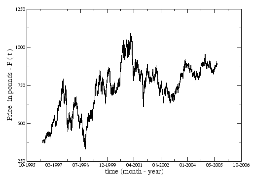
An important issue is the huge amount of data that appeared from electronic formats. Nowadays it is possible to access ![]() minute variations of prices of stocks in the market, which was impossible some decades ago. In Figure 1.1 we can see an example of the daily evolution of the price,
minute variations of prices of stocks in the market, which was impossible some decades ago. In Figure 1.1 we can see an example of the daily evolution of the price, ![]() of a company in time, in this case the bank HSBC (tick symbol HSBA) that belongs to the main index of the London Stock Exchange, FTSE100.
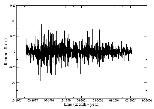
With the study of the distribution of returns of the price of a stock, some empirical results didn't match some laws used by the economics community [6,7,8]. The returns are defined as:
of a company in time, in this case the bank HSBC (tick symbol HSBA) that belongs to the main index of the London Stock Exchange, FTSE100.
With the study of the distribution of returns of the price of a stock, some empirical results didn't match some laws used by the economics community [6,7,8]. The returns are defined as:
![]() (Figure 1.2) and we use the logarithmic return for two reasons: first there is a common belief that the price of stocks,
(Figure 1.2) and we use the logarithmic return for two reasons: first there is a common belief that the price of stocks, ![]() increase exponentially, in time, on average; second is related with the fact that the difference between two consecutive prices is very small, so:
increase exponentially, in time, on average; second is related with the fact that the difference between two consecutive prices is very small, so:
| (1.1) |
 |
 |
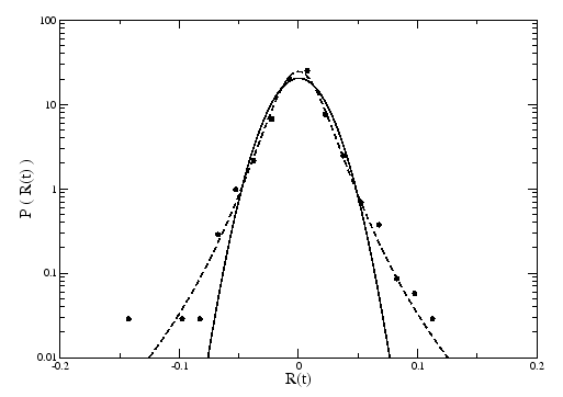 |
An important issue is thus to redevelop financial tools that were developed from Gaussian statistics, but now based on non-Gaussian statistics.
An important method frequently used for the study of time series in the stock market is Random Matrix Theory. Random Matrix Theory was previously used in Nuclear Physics to study the statistical behaviour of energy levels of nuclear reactions [9]. According to quantum mechanics, the energy levels are given by the eigenvalues of a Hermitian operator, the Hamiltonian which was postulated to have independent random elements. However, analysis of the eigenvalues of real data showed deviations from the spectra of fully random matrices, thus indicating non-random properties, useful for an understanding of the interactions between nuclei. This approach is nowadays applied to the study of correlations of time series of returns in the stock market (Section 2.2), where physicists try to find the non-random properties of the matrix of correlations [10,11,12]. With the prediction of the eigensystem of a random matrix, compared with the eigensystem of the matrix of real data of stocks, we can see eigenvalues far from the prediction spectrum, that have a lot of information about the market [13,14], as the index of the market, or the clustering in industrial sector in markets. The index of the market can be calculated as the simple mean of the prices of all the stocks that belong to the market or the weighted mean, where some stocks contribute more to the index, related with the size of the company. The industrial sectors can be different for different classifications, but normally the industrial sector means which kind of business the company is included in.
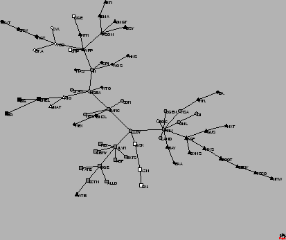
To visualise the hierarchical structure of financial markets, Mantegna defined a distance between stocks (Section 2.4.1), using the correlations between them [15]. Using this distance, he constructed a network of stocks (Minimal Spanning Tree, Section 2.4), where nodes are stocks and links are the distances between them. An example of a network of companies is represented in Figure 1.4. The relations between companies show the formation of clusters of sectors, as we can see that same symbols in Figure 1.4, are linked together. The ![]() most highly capitalised companies in the UK that comprise the London Stock Exchange FTSE100, represent approximately
most highly capitalised companies in the UK that comprise the London Stock Exchange FTSE100, represent approximately ![]() of the UK market. From these
of the UK market. From these ![]() stocks, we study the time series of the daily closing price of
stocks, we study the time series of the daily closing price of ![]() stocks that have been in the index continuously over a period of almost
stocks that have been in the index continuously over a period of almost ![]() years, starting in
years, starting in ![]() August
August ![]() until
until ![]() June
June ![]() . This equals
. This equals ![]() trading days per stock.
The legend for the symbols and industrial sectors for the data of London Stock Exchange, FTSE100 and for the World Indices data is explained in Appendix B. The tree represented in Figure 1.4 is just one example of the many trees that we already produced in our work.
trading days per stock.
The legend for the symbols and industrial sectors for the data of London Stock Exchange, FTSE100 and for the World Indices data is explained in Appendix B. The tree represented in Figure 1.4 is just one example of the many trees that we already produced in our work.
 |
Properties of the trees, like topology for different time scales [16,17], degree distribution of the nodes [18,19,20,21,22], time evolution of moments of the distances of the trees [20,21,23,24,25,26,27], spread of nodes in the tree (Section 2.4.2) [20,24,25], robustness of the tree (Section 2.4.3) [20,21,22,24,25,26,28], topology before and after financial crashes [26] and others were studied for different kinds of data [29,30].