The correlation of stock prices

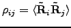
The correlation coefficient, $\rho_{ij}$ between stocks $i$ and $j$ is given by:

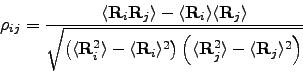$$\rho_{ij}=\frac{\langle{\bf R}_{i}{\bf R}_{j}\rangle-\langle... ...e{\bf R}_{j}^{2}\rangle-\langle{\bf R}_{j}\rangle^{2}\right)}}$$ (2.6)

where ${\bf R}_{i}$ is the vector of the time series of log-returns, 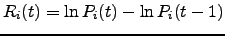$R_{i}(t)=\ln P_{i}(t)-\ln P_{i}(t-1)$ and $P_{i}(t)$ is the daily closure price of stock $i$ at day $t$. The notation $\langle\cdots\rangle$ means an average over time 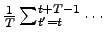$\frac{1}{T}\sum_{t'=t}^{t+T-1}\cdots$, where $t$ is the first day and $T$ is the length of our time series. We can normalise the time series of returns for each stock by subtracting the mean and dividing by the standard deviation:

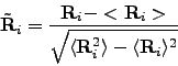$$\tilde{{\bf R}}_{i}=\frac{{\bf R}_{i}-<{\bf R}_{i}>}{\sqrt{\langle{\bf R}_{i}^{2}\rangle-\langle{\bf R}_{i}\rangle^{2}}}$$ (2.7)

The correlation coefficient is then given by: $\rho_{ij} = \langle\tilde{{\bf R}}_{i} \tilde{{\bf R}}_{j}\rangle$.

This coefficient can vary between 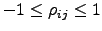$-1\leq\rho_{ij}\leq1$, where $-1$ means completely anti-correlated stocks and $+1$ completely correlated stocks. If $\rho_{ij}=0$ the stocks $i$ and $j$ are uncorrelated. The coefficients form a symmetric $N\times N$ matrix with diagonal elements equal to unity. The correlation matrix with elements $\rho_{ij}$ can be represented as:

$${\sf C}=\frac{1}{T}{\sf G} {\sf G}^T$$ (2.8)

where ${\sf G}$ is an $N\times T$ matrix with elements $\tilde{R}_{i}(t)$ and ${\sf G}^T$ denotes the transpose of ${\sf G}$.

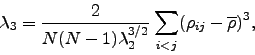
The distribution of correlation coefficients is an important aspect of our study because can show how the stocks from a portfolio are related with each other. If we compare the distribution of real data with the one made from random data (Figure 3.1), conclusions about the non-randomness of the market can be done. We can also study the moments of this distribution, as the mean [20,25]:

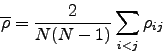$$\overline{\rho}=\frac{2}{N(N-1)}\sum_{i<j}\rho_{ij}$$ (2.9)

the variance:

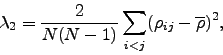$$\lambda_{2}=\frac{2}{N(N-1)}\sum_{i<j}(\rho_{ij}-\overline{\rho})^{2},$$ (2.10)

the skewness:

$$\lambda_{3}=\frac{2}{N(N-1)\lambda_{2}^{3/2}}\sum_{i<j}(\rho_{ij}-\overline{\rho})^{3},$$ (2.11)

and the kurtosis:

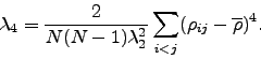$$\lambda_{4}=\frac{2}{N(N-1)\lambda_{2}^{2}}\sum_{i<j}(\rho_{ij}-\overline{\rho})^{4}.$$ (2.12)

Just the elements of the upper triangle of the matrix are used to compute the matrix, because it's a symmetric matrix with diagonal elements equal to unity. If we divide our time series in small windows and we move these windows in small steps, we create different correlation matrices, and if we compute the moments of each matrix, we can study these moments in time.