Distances

The metric distance, introduced by Mantegna [15], is determined from the Euclidean distance between vectors, $d_{ij}=\vert\tilde{{\bf R}}_{i}-\tilde{{\bf R}}_{j}\vert$. Because $\vert\tilde{{\bf R}}_{i}\vert=1$ it follows that:

$$d_{ij}^{2}=\vert\tilde{{\bf R}}_{i}-\tilde{{\bf R}}_{j}\vert... ...^{2}-2\tilde{{\bf R}}_{i}\cdot\tilde{{\bf R}}_{j}=2-2\rho_{ij}$$ (2.23)

This relates the distance of two stocks to their correlation coefficient:

$$d_{ij}=\sqrt{2(1-\rho_{ij})}$$ (2.24)

This distance varies between $0\leq d_{ij}\leq2$ where small values imply strong correlations between stocks. Following the procedure of Mantegna [15], this distance matrix is now used to construct a network with the essential information of the market.

This network (MST) has $N-1$ links connecting $N$ nodes. The nodes represent stocks and the links are chosen such that the sum of all distances (normalised tree length) is minimal. We perform this computation using Prim's algorithm [67]. The Prim's algorithm is given by:

• Choose the minimum distance between a pair of stocks and construct a link between them;
• Choose the next minimum distance between a pair of stocks, where one of the stocks already has a link but the other does not have any links. If the conditions are respected construct a link between them, if not, choose the next minimum distance where this is obeyed;
• Continue to choose pairs of stocks to link, with the conditions to verify until we reach $N-1$ links.

With the information of which stocks are connected to one another, we use the Pajek software to visualise these links [68]. The Pajek software uses the Kamada-Kawai algorithm [69] to display the links and nodes. This algorithm introduce a dynamic system in which every two nodes are connected by a ``spring'' with the respective distance between two stocks. The optimal layout of vertices is when the total spring energy is minimal. As we saw in Figure 1.4 of the Introduction, a MST of stock data is almost organised in clusters of different industrial sectors of the market.

The main idea for using MST, apart of the visualisation of links between companies, is to filter data. From the $N\times (N-1)/2$ correlation coefficients we are only left with $N-1$ points, which we believe are the most important coefficients of the correlation matrix.

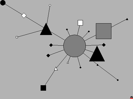
To see better this clustering property we developed a new kind of tree, where the stocks, if they belong to the same sector and are linked together, emerge in one big node. The sizes of the final nodes are proportional to the number of stocks that they contain, as shown in Figure 2.2.

Figure 2.2: New visualisation of the clusters of the MST of figure 1.4. The meaning of the symbols is explained in Appendix B.

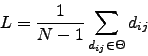
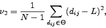
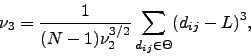
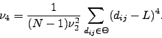
As we did for the correlations, we study the distribution of distances in the tree and the main moments, as the mean or normalised tree length:

$$L=\frac{1}{N-1}\sum_{d_{ij}\in\mathrm{\Theta}}d_{ij}$$ (2.25)

where $\Theta$ represents the MST. The other moments are the variance:

$$\nu_{2}=\frac{1}{N-1}\sum_{d_{ij}\in\mathrm{\Theta}}(d_{ij}-L)^{2},$$ (2.26)

the skewness:

$$\nu_{3}=\frac{1}{(N-1)\nu_2^{3/2}}\sum_{d_{ij}\in\mathrm{\Theta}}(d_{ij}-L)^{3},$$ (2.27)

and the kurtosis:

$$\nu_{4}=\frac{1}{(N-1)\nu_2^2}\sum_{d_{ij}\in\mathrm{\Theta}}(d_{ij}-L)^{4}.$$ (2.28)

Again we can divide our time series in small windows and move those windows in small steps, creating different MST. If we compute the moments of each MST, we can study these moments in time.