Wealth Distributions

The area of study of wealth distributions is another important aspect of economics now looked at by physicists, which is not only related with the study of wealth or income distributions in societies [3], but also with the size of companies in a country [31], or the GDP (Gross Domestic Product) of countries [32]. The study of wealth distributions has attracted great interest since the work of the socio-economist Vilfredo Pareto, who wrote a book about economical politics, $100$ years ago [33], studying a large amount of economical data (Table 1.1), he suggested that the distribution of wealth from different cities and countries follow a power law distribution with similar exponents $\alpha$ (between $1$ and $2$), known nowadays as Pareto's index:

$$P(w)\sim w^{-(1+\alpha)},\ {\rm for\ large}\ w.$$ (1.2)

The power law distribution is also known as Pareto's Law and sketches of both probability distribution and cumulative distribution are shown in Figures 1.5 and 1.6, respectively. The cumulative distribution of wealth is known as the probability that the wealth takes on a value equal of bigger than $w$:

$$C(_>w)\sim w^{-\alpha},\ {\rm for\ large}\ w.$$ (1.3)

Figure 1.5: Sketch of the distribution of income according to Pareto. For large values of income this follows a power law.

Figure 1.6: Sketch of the cumulative distribution of income. In this $log-log$ plot the power-law regime results in a straight line with slope $-\alpha$.

This work of Pareto was the first empirical study of wealth distributions, but over the last decade many physicists studied an extensive amount of data from different countries, summarised in Table 1.2.

Table 1.1: Table, taken from Pareto's book [33], showing the exponent $\alpha$ for a number of different data sets. Note that his is only a small extract of all the data that Pareto analysed.

Country

Year

$\alpha$

Country

Year

$\alpha$ England

¹ Some of the Italian main cities: Ancone, Arezzo, Parma and Pisa

Table 1.2: Table of empirical data. In column Source: S.H. - Size of Houses; I. - Income; I.T. - Income Tax; Inhe. T. - Inheritance Tax; W. - Wealth. In column Distributions: Par. - Pareto tail; LN - Log-normal; Exp. - Exponential; D. Par. - Double Pareto Log-normal; G. - Gamma.

Country

Source

Distributions

Pareto Exponents

Ref. Egypt

¹ Related to the size of houses found in an archaeological study.

² This value is an average Pareto exponent.

³ $\alpha$ and $\beta$ are Pareto exponents for the richest and poorest part, respectively.

⁴ Both distributions are a good fit of the data.

⁵ $125$ wealthiest individuals in India.

⁶ $400$ wealthiest people, by Forbes.

⁷ Top wealthiest people, by Forbes.

⁸ Top wealthiest people, by Sunday Times.

Apart from the study of the empirical data, physicist are very interested in modelling wealth distributions [34]. A detailed review of some models and open problems in the study of wealth distribution [35] was published by us in a chapter of an Econophysics book [4]. Models used in biological systems like Lotka-Volterra models, were used by physicists to explain the economic trade relations in communities [36]. Gas models of collisions were transformed into economic models where agents substitute molecules, money substitutes energy and trade substitutes collisions [37,38]. A model of dynamical network of families [39], where each node is one family and links between nodes means family relations, were used to implement money exchange between different families due to payments of new links (like weddings), payments to the society (to rear a child), distributions of money from nodes that will disappear (inheritance). 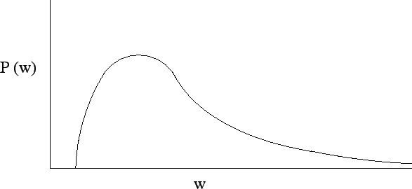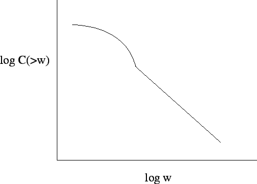The appeal in using all these models is that they are simple models, with an analytical solution, few parameters and the final result for some parameters can fit the real data of wealth distributions. But there is still parts of the distribution of wealth that are not explained completely. For example, the power law distribution of the wealth just appear for the upper $5$-$10\%$ of the society. The other part of the society is normally defined to have a log-normal or Gibbs distribution (Table 1.2). But even the power law in the end of the distribution seems to have more than one Pareto exponent. As we can see from Table 1.2 when the distribution of wealth is just related with the top billionaires, the exponent is low, compared with the top richest of the society in the other studies. A model able to explain an exponent for the rich members of the society and other exponent for the billionaires that normally appear on the list of World Top Richest (like Forbes [40]) is our goal for this project, in the future, in terms of wealth distributions.