Studying the eigensystem of the correlation matrix, we can see some financial information in the eigenvalues of the matrix and in the respective eigenvectors. We know that comparing the spectrum of eigenvalues of correlation matrix with the spectrum of eigenvalues of a random matrix, we can extract information about the market and about the sectors that constitute the market. A random matrix is defined by [63]:
| (2.13) |
 |
(2.15) |
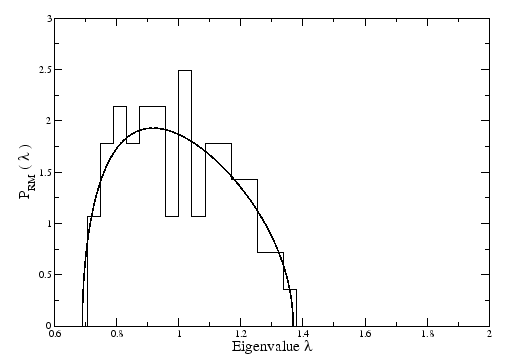 |
If we compare the results of a correlation matrix constructed with real time series, with the random matrix (Figure 3.3) we can see that the highest eigenvalues of the real matrix are much higher than the highest eigenvalue of random matrix. The largest eigenvalue represents something that is common to all stocks. If we analyse the respective eigenvector, all the stocks have the same sign (Figure 3.4), so all participate in the same way.
The largest eigenvalue and its corresponding eigenvector can be interpreted as the collective response of the market to any external factors, so it can be compared with the market index [13,14]. A way to prove this is to see the correlation between the index of the market and the projection of the time series in the eigenvector related with the largest eigenvalue (Figure 3.5). The projection is given by:
If we filter the real time series, extracting the market mode from every stock, we get a new correlation matrix with the residuals ![]() [14]. A way to filter the market mode is to use the one-factor model or Capital Asset Pricing model [64], where the return of the price can be expressed as:
[14]. A way to filter the market mode is to use the one-factor model or Capital Asset Pricing model [64], where the return of the price can be expressed as:
| (2.17) |
 |
(2.18) |
The residuals are given by:
If we analyse the spectrum of eigenvalues of the new filtered matrix, some eigenvalues continue to be far outside the range obtained from equation 2.14 . These are the eigenvalues that represent different sectors. Our main work is to try to understand a way to filter this information, to end up with a time series of random information. Our approach is to use a multifactor model, where we not just use a market mode, but also a sector mode [65,66]. This sector mode is defined for each sector in our portfolio and is related with the highest eigenvalue of the correlation matrix of the stocks of only one sector, similar to what we did for the whole market. Our multifactor model can be represented as:
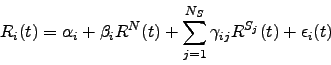 |
(2.20) |
 |
|||
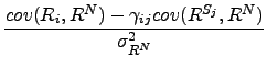
![$\displaystyle \frac{cov(R_i,R^{S_j})\sigma_{R^N}^2-cov(R_i,R^N) cov(R^{S_j},R^N)}{\sigma_{R^{S_j}}^2 \sigma_{R^N}^2 - \left[cov(R^{S_j},R^N)\right]^2}$](img191.png) |
(2.22) |
We will need to check if this model is enough to represent the returns of the stocks, or if there are other terms, like for example a term of correlations between stocks of different sectors.