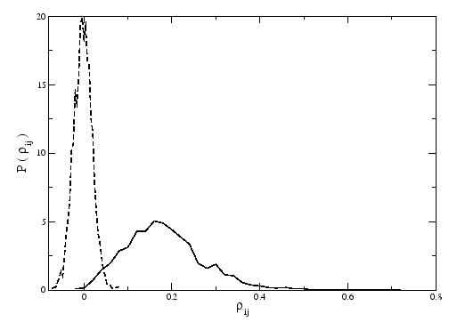
The distribution of coefficients of the correlation matrix constructed from the time series of stocks of the FTSE100, is shown in Figure 3.1 and compared with the distribution of coefficients of a correlation matrix of shuffled time series. The results of the shuffle time series are similar with the one for random time series, because the correlation in time of different companies is destroyed. As expected for a random matrix, the distribution of the coefficients for the shuffle time series is symmetric and with zero mean, different from the original time series, where the distribution is asymmetric with non-zero mean. But the distribution depends on the length ![]() of the time series and depends on external aspects that affect the market as we can see in Figure 3.2. If we divide our time series in small windows and we move these windows in time, we will get different matrices of correlations and different distributions of the coefficients. We do this in order to see the market changes. We choose to divide the time series in windows of size
of the time series and depends on external aspects that affect the market as we can see in Figure 3.2. If we divide our time series in small windows and we move these windows in time, we will get different matrices of correlations and different distributions of the coefficients. We do this in order to see the market changes. We choose to divide the time series in windows of size ![]() days and move them day by day, so we will get
days and move them day by day, so we will get ![]() (
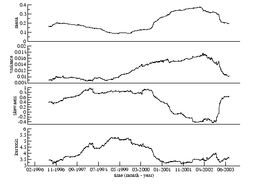
(![]() ) different matrices. In Figure 3.2 we can see the moments of the distribution of coefficients in time where the mean and variance are highly correlated (
) different matrices. In Figure 3.2 we can see the moments of the distribution of coefficients in time where the mean and variance are highly correlated (![]() ), the skewness and kurtosis are also highly correlated and the mean and skewness are anti-correlated. This implies that when the mean correlation increases, usually after some negative event in market, the variance increases. Thus the dispersion of values of the correlation coefficient is higher. The skewness is almost always positive, which means that the distribution is asymmetric, but after a negative event the skewness decreases, and the distribution of the correlation coefficients becomes more symmetric.
), the skewness and kurtosis are also highly correlated and the mean and skewness are anti-correlated. This implies that when the mean correlation increases, usually after some negative event in market, the variance increases. Thus the dispersion of values of the correlation coefficient is higher. The skewness is almost always positive, which means that the distribution is asymmetric, but after a negative event the skewness decreases, and the distribution of the correlation coefficients becomes more symmetric.
 |
 |