


Next: The correlation of stock
Up: Methods
Previous: Methods
Contents
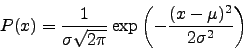
As we already said in the Introduction, some economists assume the returns to be Gaussian distributed, but we saw in Figure 1.3 that the tails of the distribution are ``fatter'' than a Gaussian distribution. To fit the Gaussian distribution we computed the mean ( ) and standard deviation (
 ) of the returns and plotted the probability distribution function:
 |
(2.1) |
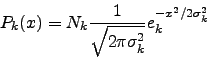
But we can fit distributions with fat tails, like the T-student or Tsallis distribution [61] to the distribution of returns and see if the tails are better fitted with this. The probability distribution function of a T-student is given as:
 |
(2.2) |
where  is a normalisation factor:
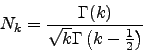 |
(2.3) |
and
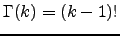 is the Gamma function. The factor
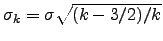 is related with the effective standard deviation of the distribution () and with the degree of distribution (
 ). The function
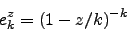
  is an approximation of the exponential function called k-exponential:
 |
(2.4) |
and in the limit
 this function reduces to the ordinary exponential function. The probability distribution function can be written as:
![\begin{displaymath}
P_k(x) = \frac{\Gamma(k)}{\Gamma \left( k-\frac{1}{2}\right)...
...2 k -3)}} \left[1 + \frac{x^2}{\sigma^2 (2 k -3)} \right]^{-k}
\end{displaymath}](img121.png) |
(2.5) |
The parameter is related with the Tsallis parameter  by
by 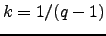 . The computation of the parameters of T-student distribution is explained in Appendix A.
For all the stocks of the London Stock Exchange that we studied, the minimum value of is
. The computation of the parameters of T-student distribution is explained in Appendix A.
For all the stocks of the London Stock Exchange that we studied, the minimum value of is  and the maximum
  , but most of the values are in the
 ![$[2, 4]$](img126.png) interval, which means values of in the
interval, which means values of in the ![$[1.25, 1.5]$](img127.png) interval, that is around the values found by Tsallis [62] (
interval, that is around the values found by Tsallis [62] ( ,
,  and
and  ) for
) for  ,
,  and
and  minutes return, respectively, for the NYSE in 2001. For example the value of found for HSBC company is
  (the one used in the T-student distribution in Figure 1.3).
Our study is based on the assumption that the returns of the stock price carry more information than random noise. To check this, we will compute the correlation between returns of stock prices and analyse the correlation matrix. The main idea of our work is to find the underlying correlation matrix of stock returns.
Next: The correlation of stock
Up: Methods
Previous: Methods
Contents
Ricardo Coelho
2007-05-08