Creating New Materials from 2D Monolayers
Monolayer Calculations
As the title suggests, the aim of the project was to create new materials by stacking layers of different 2D nanomaterials. Well actually we created them theoretically and then investigated their properties to see if it is possible for them to exist in nature. It's easier said than done though because the different materials need to have similar crystal structers and lattice constants. I had to run calculations to work out the binding energies of different materials and how much stress could be applied to a layer, because if two materials are relatively soft, then the monolayers can be streched / compressed to bring the lattie constants as close to each other as possible. Of course the energy required to apply this stress has to be compared to the binding energy of the material to see if it is energetically favourable. The amount of stress that can be applied to a layer is around 0.2% at the best of times... Here is an example of the typical calculations that I ran for such materials: GeI2 is one of the softer materials and thus it is more likely that it can be combined with other materials.
GeI2
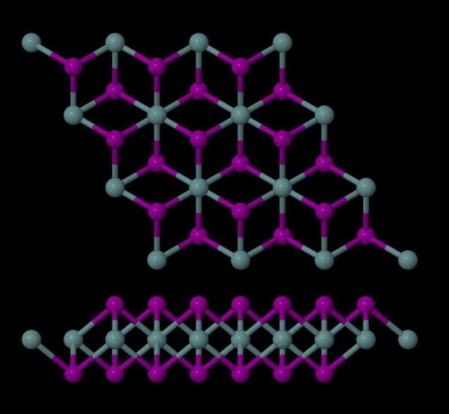


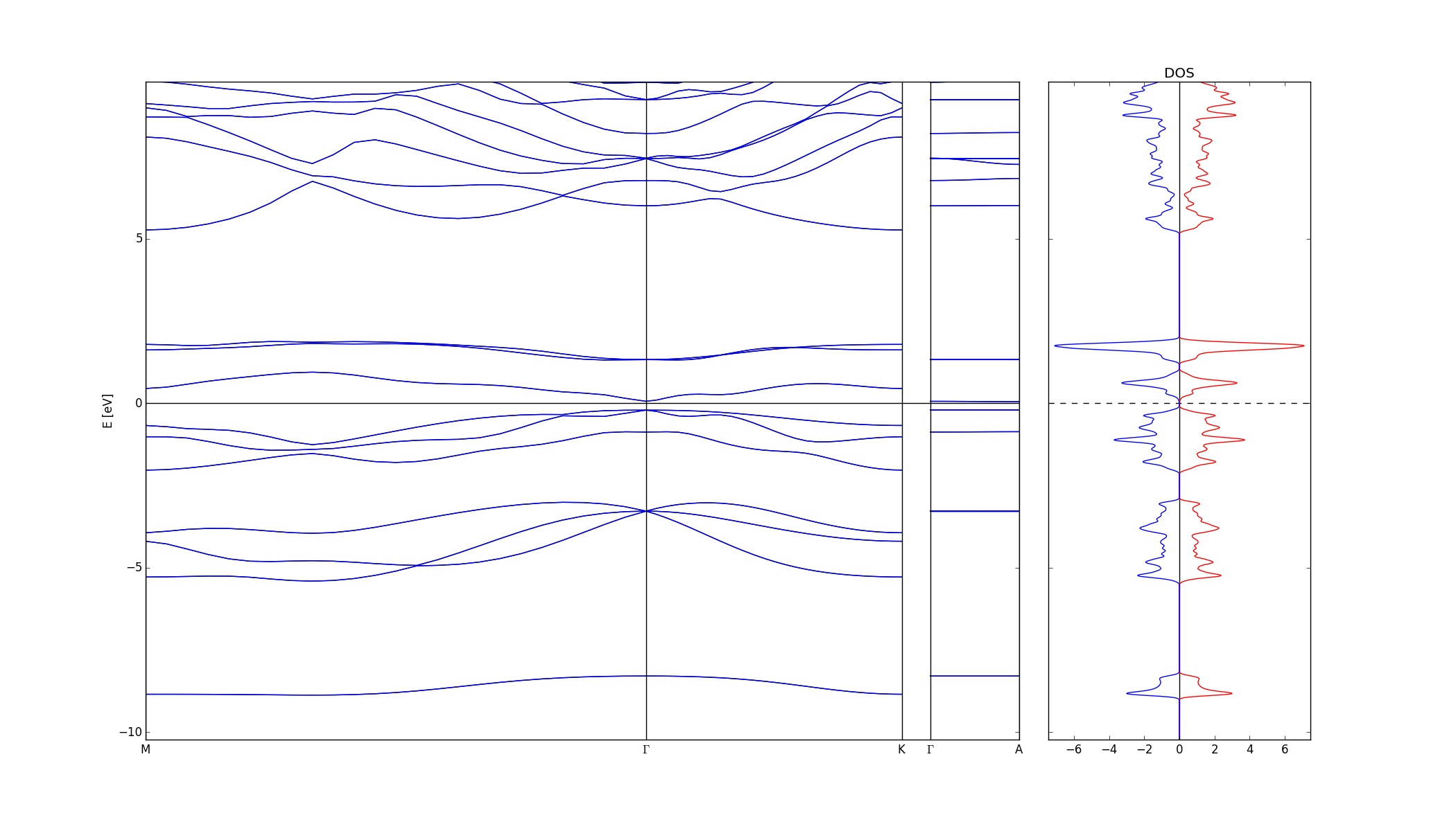
The first figure is a stress calculation. Plotted is the change in energy (eV) against stress (%). A parabola is nicely fit to the data, and the width of the parabola indicates how susceptible a material is to applied stress. The second figure plots the energy of the monolayers versus the layer separation. The data is (badly) fit with an interpolation function, but it gives the nice shape of an interaction potential. The bottom of this well gives the optimal layer separation for the system. The third figure is a band structure and density of state calculation. The first two sections of the band structure are along directions that lie in the plane of the monolayer, so they show the interlayer interactions. The final section is along the direction perpendicular to the plane. The flat lines indicate that there is no interaction between layers
The three materials of interest were GeI2, SnS2 and SnSe2, but a more detailed page of monolayer calculations for many materials can be found here here.
Combining the Layers
The next step was to start combining the layers. My calculations required a geometry file and a control file; there is a database of geometry files for different materials but for the bilayers I had to make them by hand, since there hasn't been much work done on them yet. Here's a few examples of the combined bilayers:
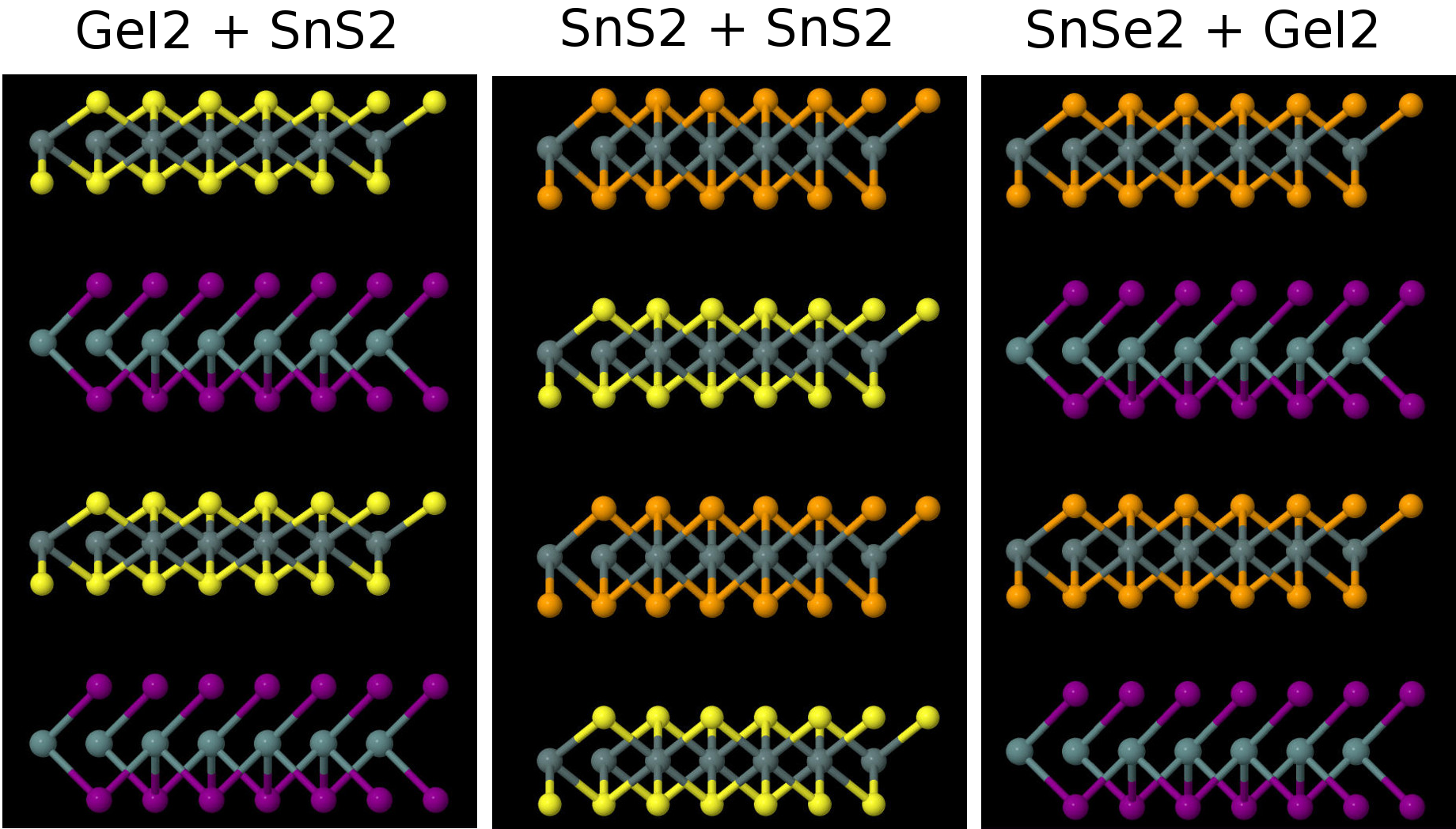
Since I constructed these configurations manually, they had to be relaxed. This means all of the atoms are moved around slightly until they find the most comfortable configuration. For the lattice constants, I just used the average lattice constants of the two materials in isolation, so I expected that to change a bit after relaxation. I also found the optimal layer separation distance exactly as before.
Sliding the Layers
With the bilayers successfully created, the next problem was finding the best way to geometrically combine two layers. This can be done in two ways: either slide one layer on top of the other or rotate one layer with respect to the other until the configuration that minimizes energy is obtained. I went with the first option, because it can be done with unit cell (6 atoms) calculations. A postdoc in the group is doing the rotational calculations, because they require supercell calculations; these require defining a large unit cell from several primitive cells, and the calculations can take weeks since there is such a large number of atoms...
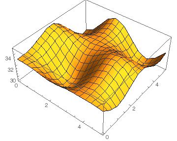
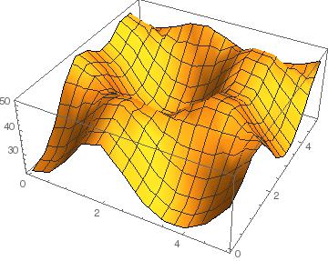
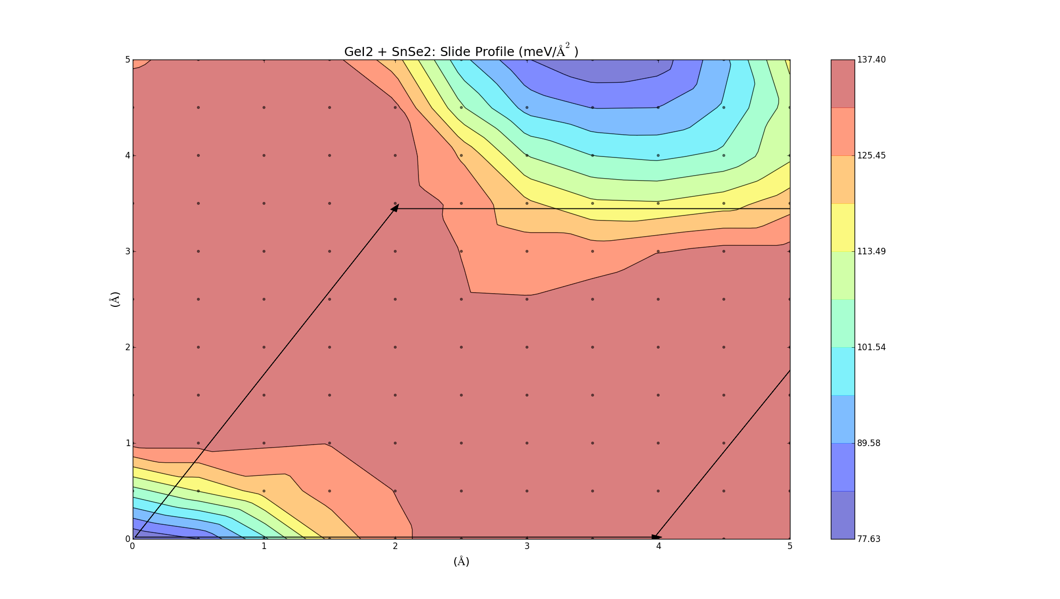
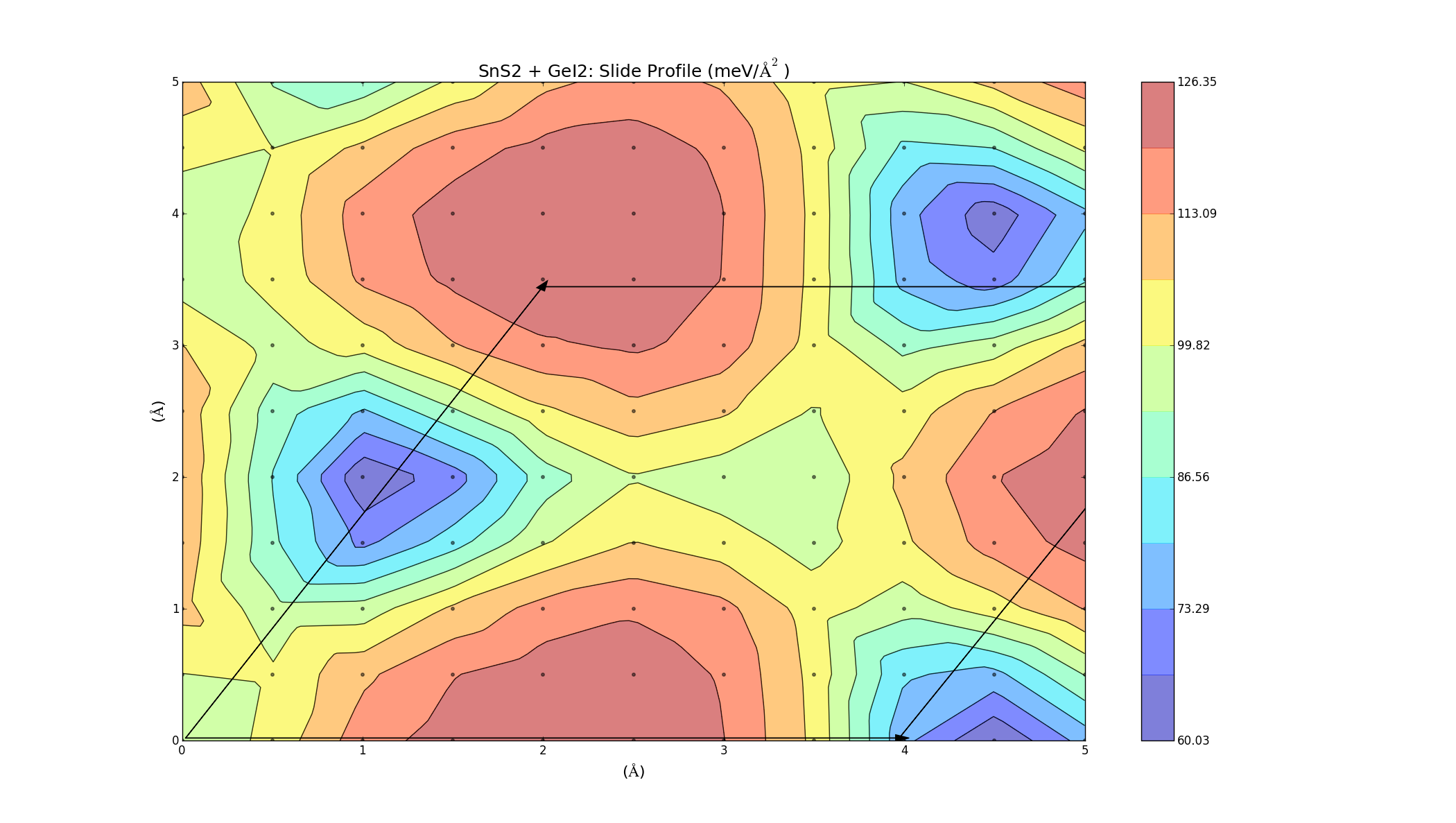
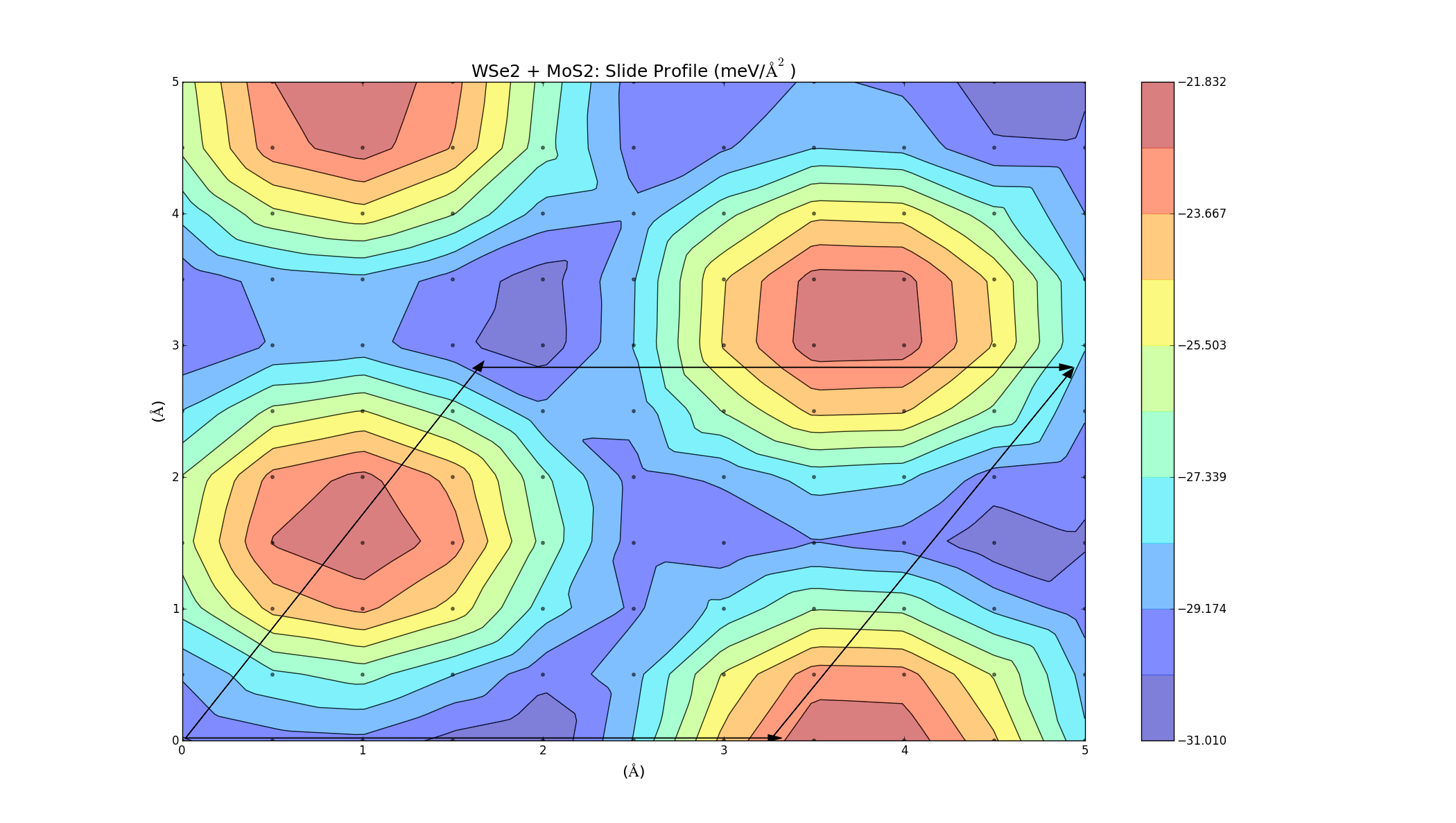
To find the best way to combine the layers, one was slid on top of the other, creating an energy profile on a 5Å x 5Å grid. This was done for the three bilayers (which took a lot longer anything else, each graph was a 2D grid with over 100 points) and the results varied for each combination. The colour represents the binding energy of the system per unit area. A negative binding energy means that the system is stable, and a positive binding energy indicates that the materials won't combine. The arrows represent the unit cell (hexagonal) for each system.
GeI2 + SnS2
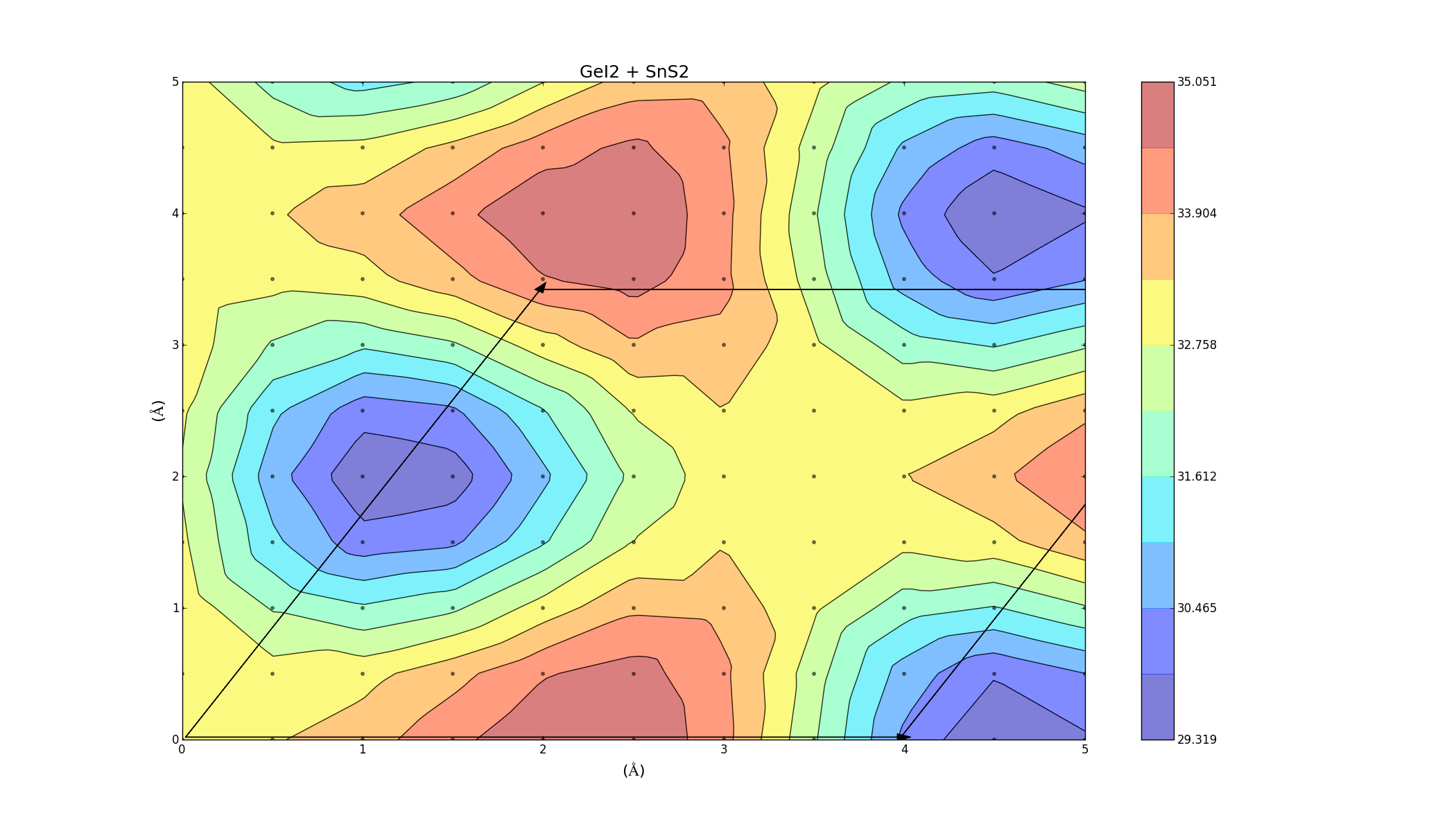
Here we see that no point on the contour has a negative binding energy, which indicates that the layers won't combine. There is a relatively low barrier height of around 6 meV/Ų. This is the energy needed to get from one minimum another in the most efficient way (moving around the red maximum through the yellow region).
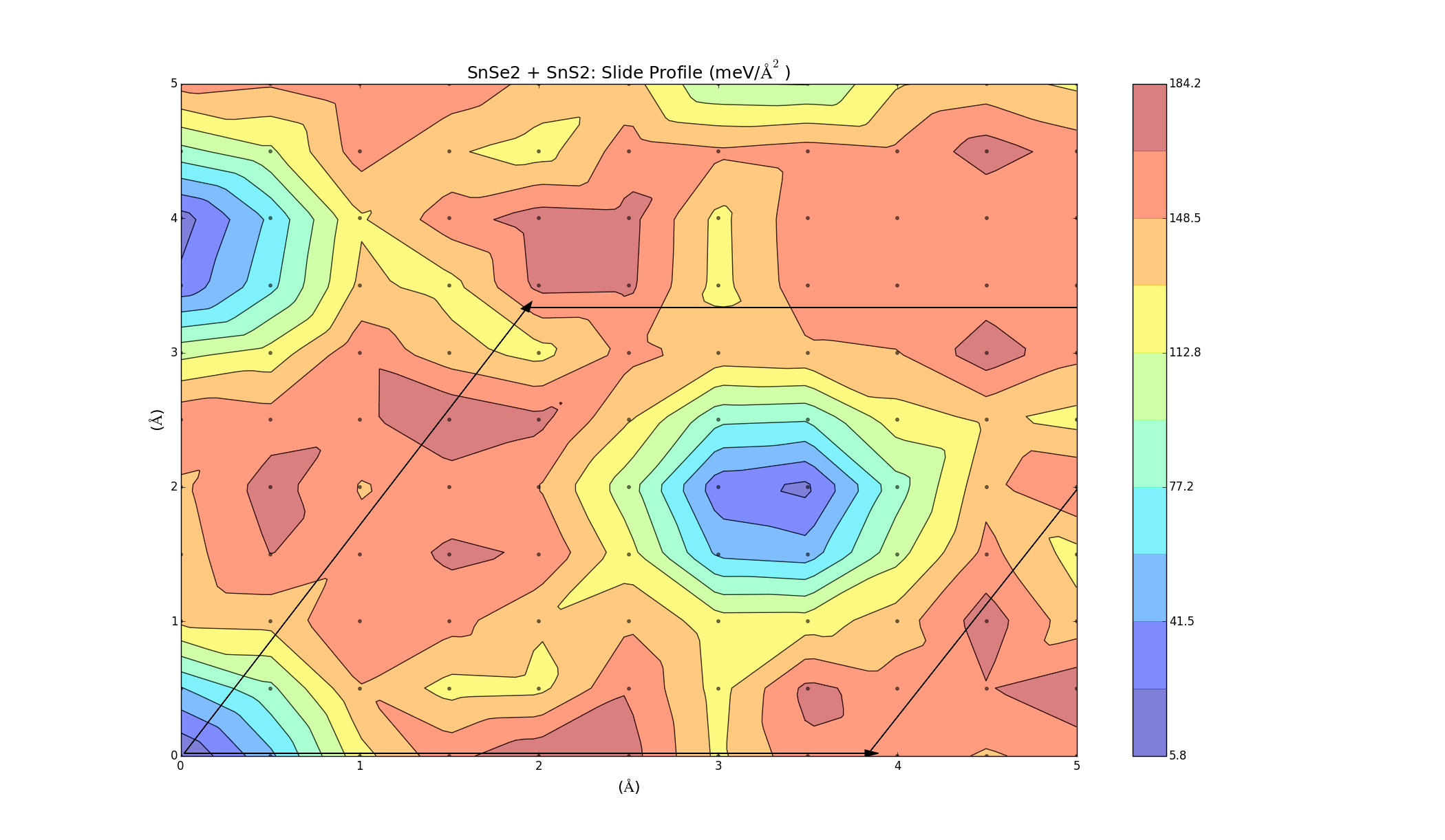
SnS2 + SnSe2
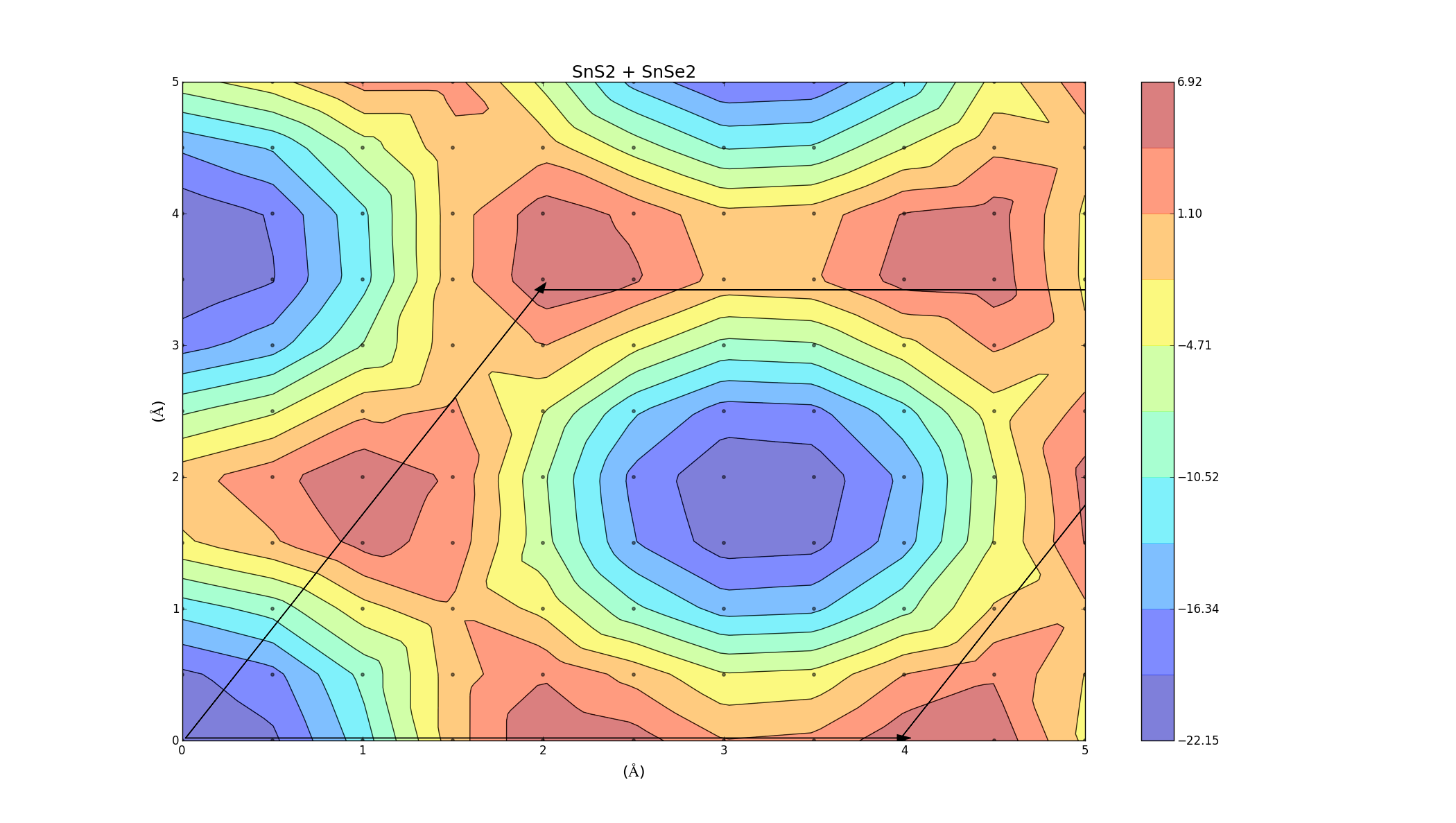
Here we see that the plot shows a primarily negative binding energy, indicating that the layers can combine. There is a barrier height of about 20 meV/Ų though.
SnSe2 + GeI2
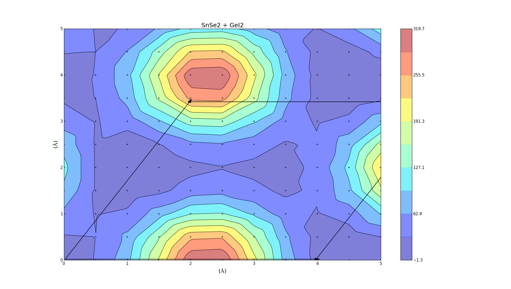
Again we see that there are parts of this plot with negative binding energy, but there is still a barrier height to overcome.
Polymorphs
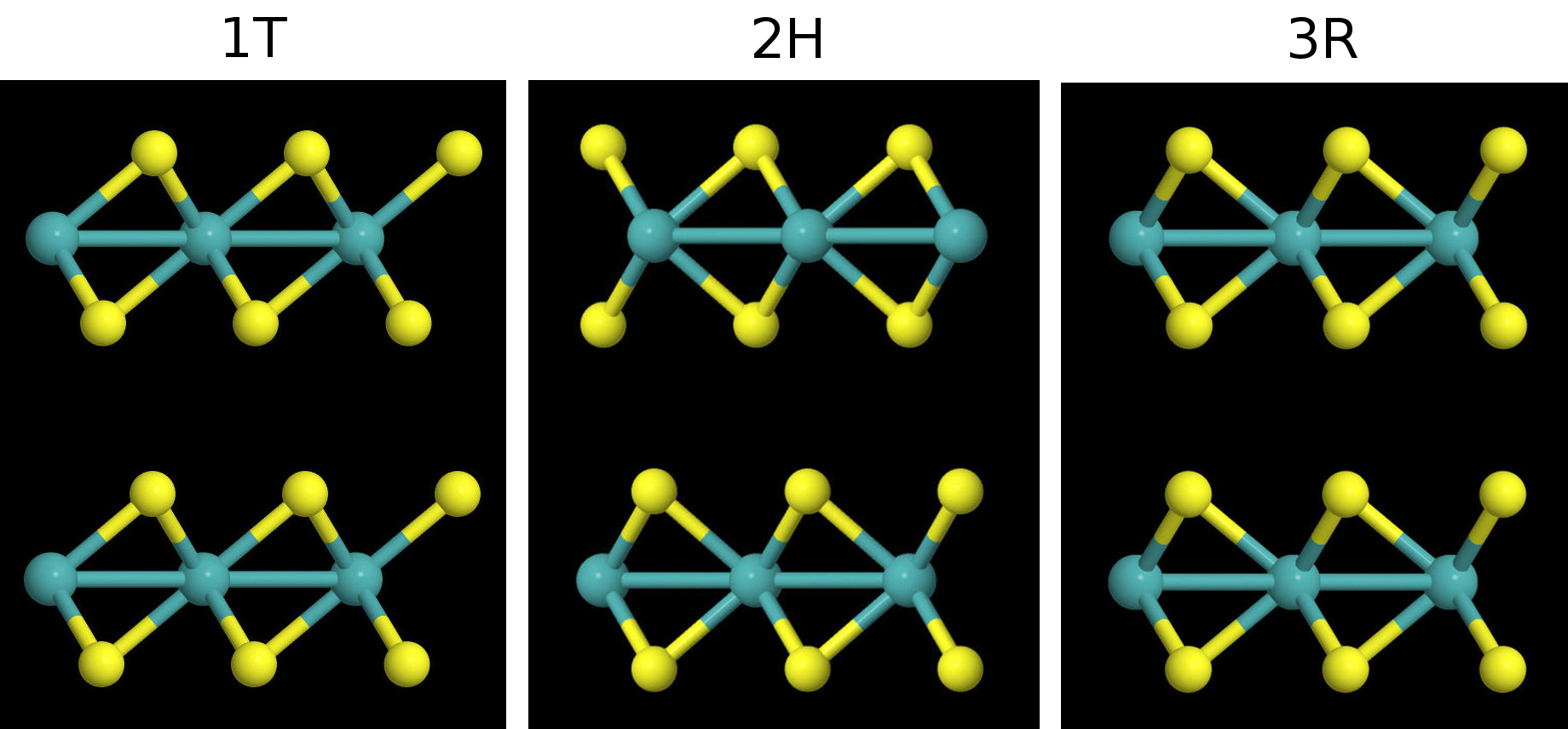
Most of the materials we are working with are hexagonal, but there are different polymorphs for each material and different ways to stack the layers with respect to one another. Each polymorph has a different space group and different associated binding energy. I compared the binding energies for different polymorphs (1T, 2H, 3R) of several different materials. Here's a side view of the hexagonal MoS2 bilayers for the 1T, 2H, 3R polymorphs. Note: only the 2H and 3R polymorphs are found in nature for this material, I constructed the 1T, polymorph myself.
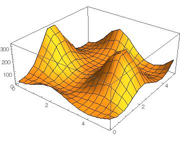
The following graph compares the binding energy for the different polymorphs of MoS2. The graph is in units of meV/Ų and the energy of the last point on the graph (taken to be the energy of the layer on its own) has been subtracted from the rest of the data points, so the graph shows binding energy per unit area as a function of distance. The different polymorphs all have the shape but with different minima, and as the layer separation distance gets larger they all approach the same value, which is good. The 3R polymorph has the shallowest well and the largest separation. The 1T has the deepest well, possibly because it doesn't exist in nature (or maybe that's why it doesn't exist in nature).

Sliding the Layers: Round 2
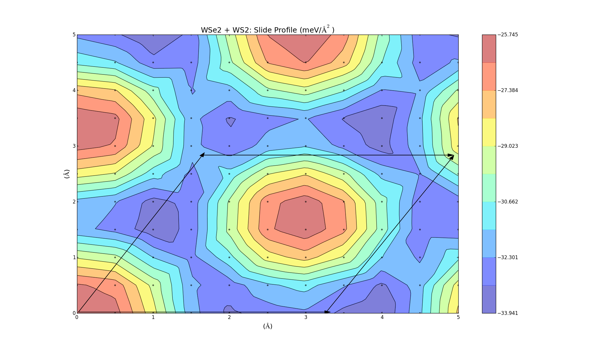
The barriers on the slide profiles don't actually have to be traversed. The calculations were a simplified approximation, and while they are nice and illustrative, they don't take into account that the layer separation distance can change slightly as one layer slides over the other in order to minimise energy. Currently I'm on redoing the slide calculations, but allowing the 2 layers to relax in the z-direction at each point to get a more accurate energy profile. I'm currently doing this for layers of the same material (MoS2, WS2, Graphene), but the results will take a while as the calculations are quite large. Once those are done I will hopefully be able to redo the combined bilayer calculations and get a better indicator as to which materials can be combined.
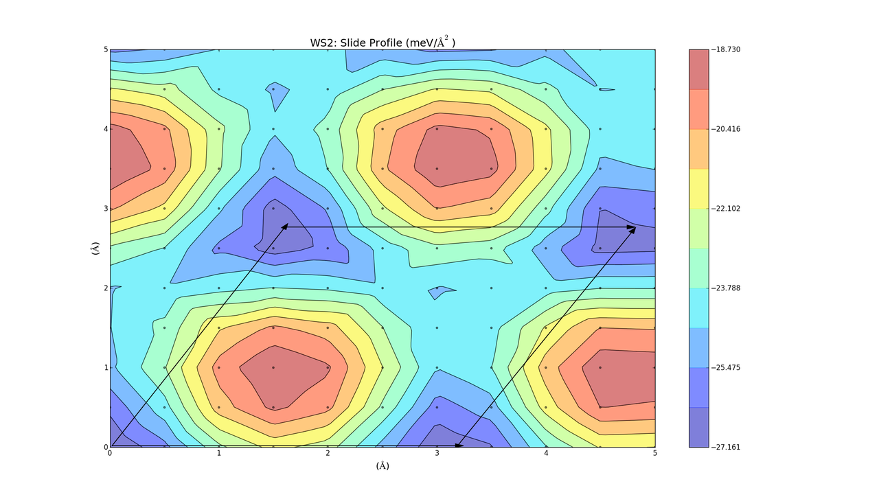
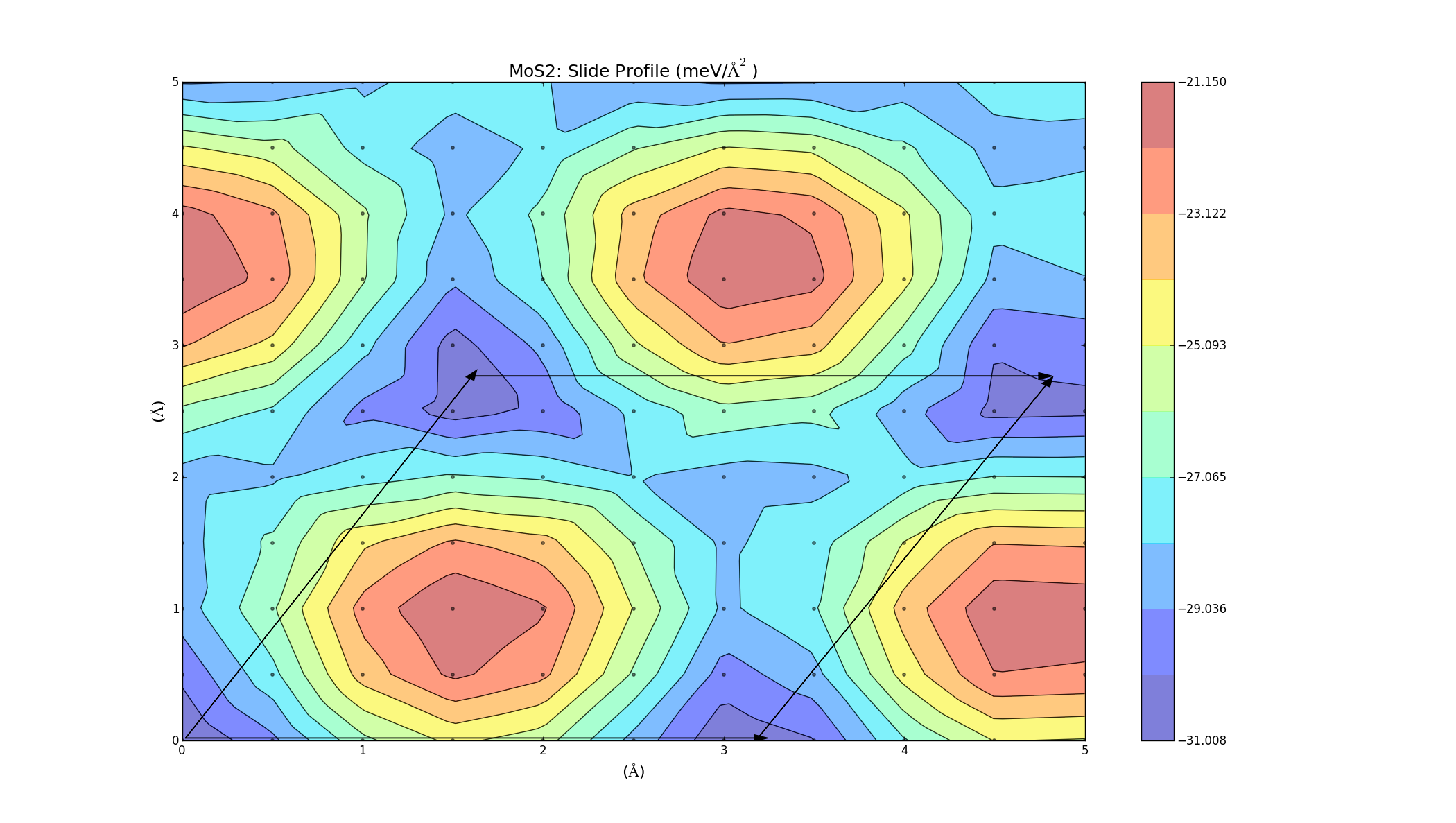
These turned out really well. Every point on the graph has a negative binding energy, and there is a low barrier height. Although these calculations were for two layers of the same material, so it makes sense that they turned out well (If you want to see the graphs in better detail, just right click and select view image).
This process was then automated and applied to layers of different materials. The unit cell for the two layers is created, and then a full unit cell relaxation and geometry optimisation is preformed. One layer is then slid over the other, and at each point it can relax in the z direction; this should give a more accurate slide profile.
An elastic analysis was preformed for combinations of different materials, and only the materials that were predicted to combine from that were considered, since the slide calculations take a long time to compute (each graph has 121 points which take about 5 hours each to compute). For the two layers, the stress parabola is plotted about the lattice constant of each material, and a new parabola formed by the superposition of the two is obtained. The minimum of this parabola will give the lattice constant and binding energy of the combined layers: if the minimum of this parabola is below zero then they should in theory combine:
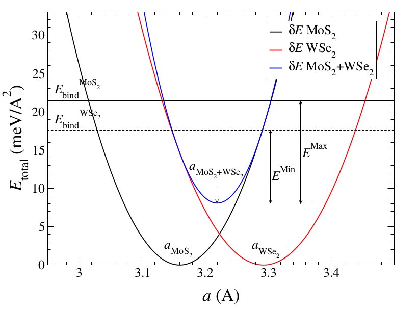
In this example, the binding energy of the new parabola is less than the binding energy of the two materials, indicating that they will combine. In all of these calculations, the binding energy is defined as the energy of the bilayer minus the energy of the two individual layers, so a negative energy means they will combine and a positive energy means they won't. The stress calculations from before were used to create plots like this, and a 2d table of binding energies for different combinations of materials was formed. The slide calculations were then preformed for the combinations with negative binding energies.
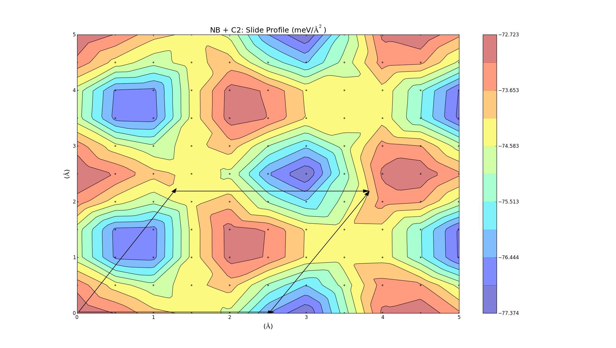
The results for the refined slide calculations were varied. Some of the graphs turned out very nice and indicated that the materials would bind, but some of them contradicted the previous calculations; I have a feeling that if there is a mistake, it is probably in the older calculations, though. One thing I noticed is that I wasn't accounting for the energy used in applying stress to the two layers to change their lattice constants. I used the coefficients from the stress parabolae together with the change in lattice constant to account for this energy. There was also a geometry factor of √3 because of the hexagonal structure of the layers. This did lower the energy in all cases, but overall the results are not consistent with the elastic binding analysis (yet). Here is the slide profile for NB + C2 bilayers:
I will keep a table of results here and update it as the calculations finish (there are a lot of them and they take a long time to compute). Hopefully I will also figure out if there's something I'm not accounting for too.
| SnSe2 | NB | MoS2 | SnS2 | C2 | MoSe2 | NbSe2 | WS2 | GeI2 | WSe2 | |
| SnSe2 | 5.8 | 80.360 | 77.63 | |||||||
| NB | -77.374 | |||||||||
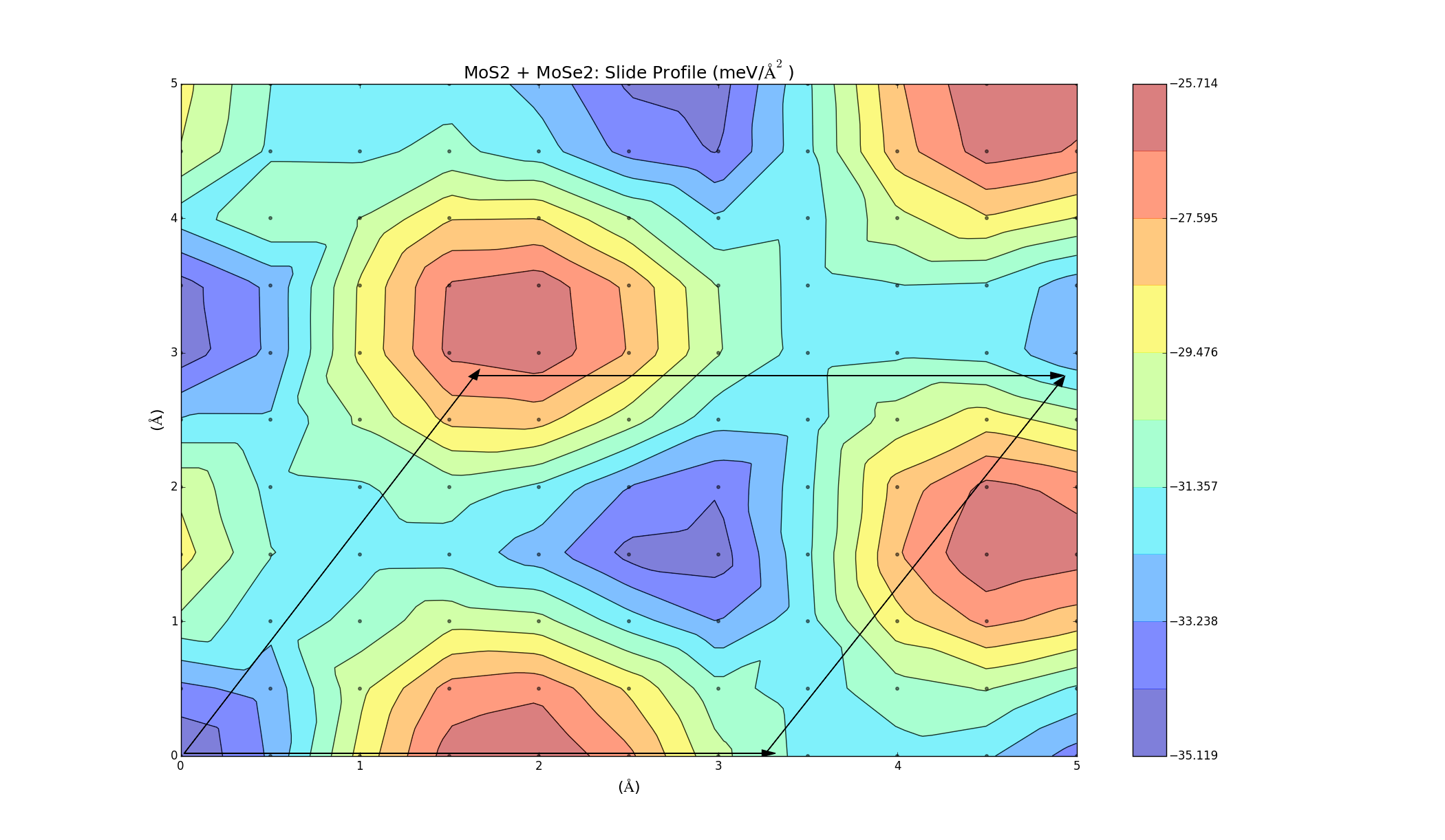
| MoS2 | -35.119 | -41.670 | ||||||||
| SnS2 | 5.8 | 0 | 60.03 | |||||||
| C2 | -77.374 | |||||||||
| MoSe2 | -35.119 | -35.010 | ||||||||
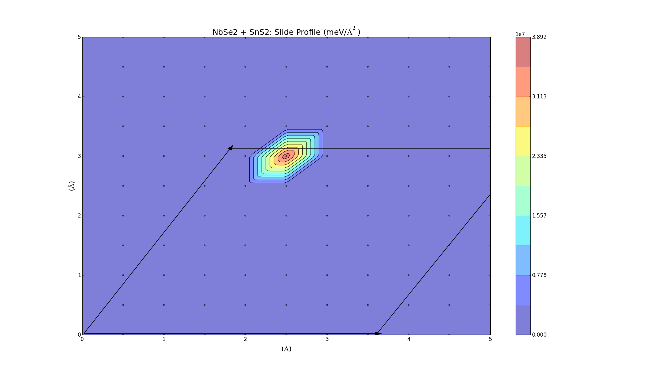
| NbSe2 | 80.360 | 0 | ||||||||
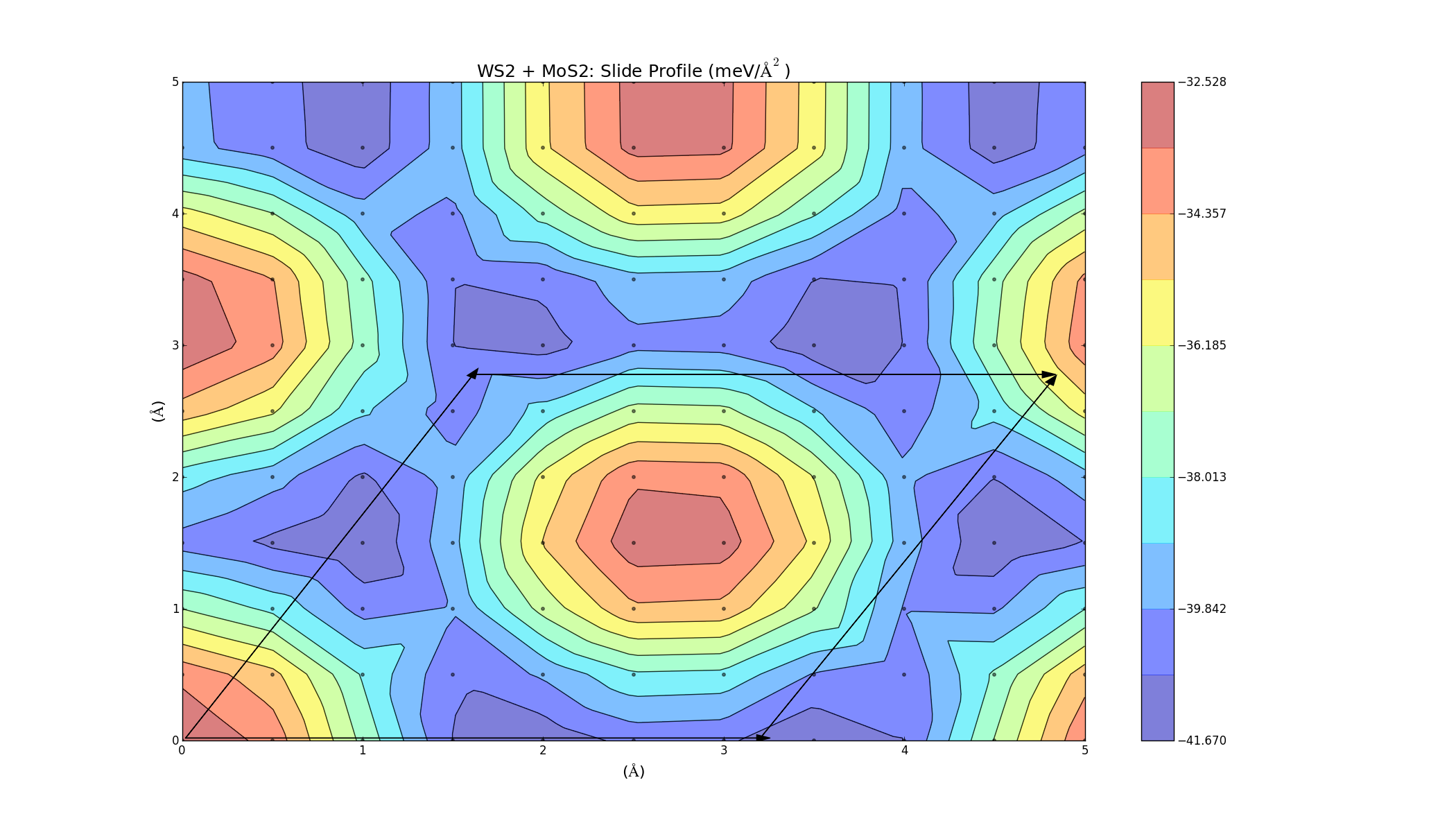
| WS2 | -41.670 | -35.010 | -33.941 | |||||||
| GeI2 | 77.63 | 60.03 | ||||||||
| WSe2 | -33.941 |
One reason that the contour plots aren't consistent with the elastic binding analysis might be that applying stress to the system has a more complex effect than originally thought.
Binding Energy vs Stress
The relationship between binding energy and stress for a bilayer system was investigated. To do this, a stress was applied the MoS2 bilayer, and then a relaxation in the z-direction was preformed to minimise the energy with respect to layer separation. The energy of the monolayer at each percentage of stress was also calculated. This was subtracted twice from the energy of the bilayer, (one for each layer) giving the binding energy as a function of stress. What was interesting is that the shape of the curve depends on the definition of "per unit area". Taking the unit cell area of the strained system for each point results in a linear relationship, whereas taking everything with respect to the unstrained unit cell area results in a quadratic relationship:


Polymorphs: Round 2
I think I misinterpreted the goal of the polymorph calculations the first time around. The idea wasn't to look at the binding energy curves of each polymorph; that doesn't make sense because some of them don't exist in nature. The goal was to take the polymorphs that do exist in nature and look at the binding energy curves of the different ways they can be stacked. The difference between the highest and lowest binding energy curves is effectively the amount of energy that can be saved by stacking the layers efficiently. Here's an illustration for the 2H/3R and 1T polytypes:
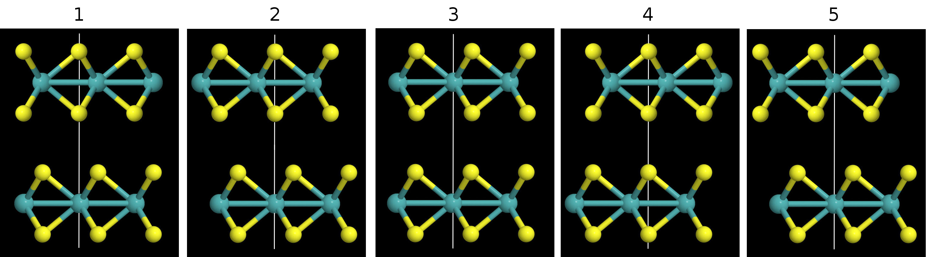
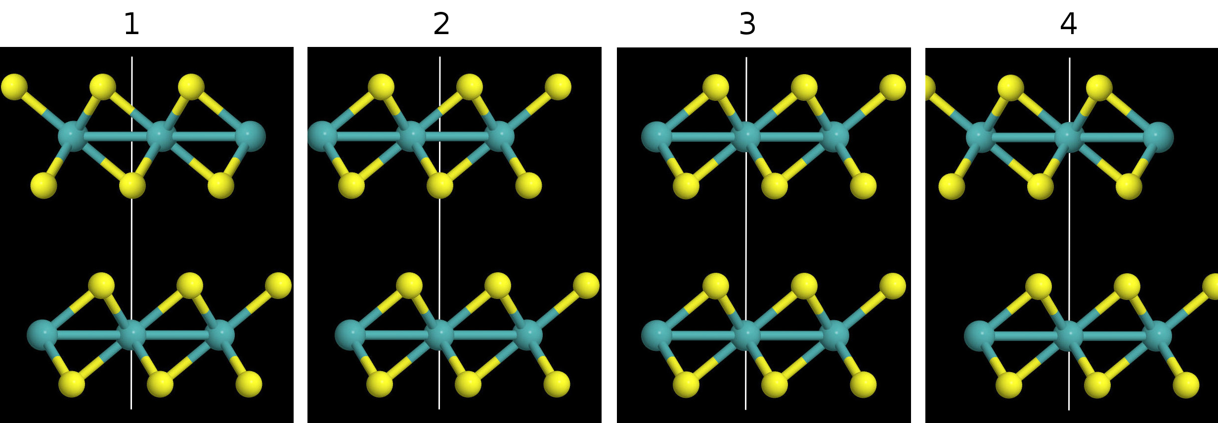
From the diagrams it can be seen that the different arrangements are obtained by aligning different atoms in the layers, as indicated by the white lines.