(2.16)
(2.17)
Density functional theory (DFT) is an ab initio approach to the calculation of materials’ properties on the atomic scale, in that it is derived from first principles without assumptions e.g. fitting parameters based on experimental evidence. However, due to its complex nature, certain justified simplifications are made in order to allow calculations to be performed with a reasonable speed.
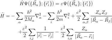
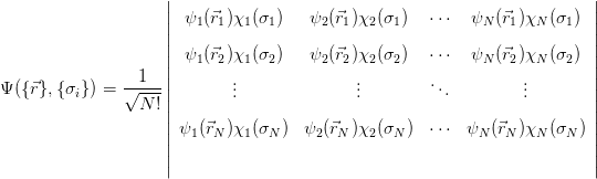
To perfectly simulate the properties of a material, one must solve the Schrödinger equation (Equation 2.16) for all the material’s electrons and nuclei. The Hamiltonian for this system is given in Equation 2.17, with the first two terms describing the kinetic energies of the nuclei and electrons, respectively, and the following terms the internuclear, electron-electron and nucleus-electron Coulomb interactions.
| (2.16) (2.17) |
For N electrons and M nuclei, this leads to a non-separable partial differential equation with 3(M + N) variables, which is obviously impossible to solve in practice for all but the simplest systems.
Instead, the Born-Oppenheimer (BO) approximation states that since the ratio of the mass of a nucleon to that of an electron Mn∕me ≈ 1836, nuclei move much slower than electrons, and so can be regarded as static; i.e. their kinetic energy term can be neglected. In this way, the molecular wavefunction is split into an electronic and a nuclear term:
 | (2.18) |
The BO Hamiltonian for the electrons therefore becomes:
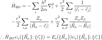 | (2.19) |
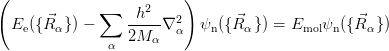
The nuclear kinetic energy is then reintroduced into the Schrödinger equation for the nuclear motion:
 | (2.20) |
Implicit in the BO approximation is the idea that electrons which interact with each other merely move in a fixed potential created by the nuclei, and that no electronic transitions occur as a result of the (slow) nuclear motion. Unfortunately, even the decoupled equation is a very complicated interacting many-body problem and still contains 3N variables.
In 1927, just one year after the publication of the Schrödinger equation, Douglas Hartree proposed a formalism to describe many electron systems. In the Hartree approach, the many-body wavefunction is replaced by the product of the wavefunctions of the individual electrons:

Applying this wavefunction to Equation 2.19, and minimising the energy while constraining the wavefunction to be normalised leads to the Hartree equation:
 | (2.21) |
Unfortunately, in 1930, J. C. Slater and V. A. Fock pointed out that the Hartree method did not conserve the antisymmetry of the wavefunction, and so the more complex Hartree-Fock approximation was developed.
Taking an ansatz for  where the Slater determinant guarantees that the
Pauli principle is respected and the wavefunction is antisymmetric upon particle
exchange:
where the Slater determinant guarantees that the
Pauli principle is respected and the wavefunction is antisymmetric upon particle
exchange:
 |
 ,
and gives rise to an integral-differential equation, which is more computationally
intensive to solve than the Hartree approximation.
,
and gives rise to an integral-differential equation, which is more computationally
intensive to solve than the Hartree approximation.
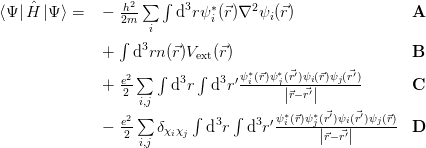
The eigenvalues of ψi are Lagrange multipliers, and can be interpreted as an approximation to the electron’s ionisation energy under the approximate assumption that the other orbitals are unaffected.
The “Hartree” term simplifies to:
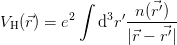 | (2.22) |
 ) = ∑
iψi∗(
) = ∑
iψi∗( )ψ
i(
)ψ
i( ) is the full charge density. This realisation leads
to the fundamental idea behind density functional theory. If the full wavefunction
was used, the amount of memory required to store it grows exponentially with N.
For example, if it were represented on a very rough grid, with 3 points per degree
of freedom, the amount of memory scales as roughly ∼101.5N, so for just 50
electrons, ∼1075 values would need to be stored (for comparison, the number of
baryons in the observable universe is ∼1080). Instead, in their seminal 1964 work
Pierre Hohenberg and Walter Kohn proposed that it is sufficient to avoid the full
many-body wavefunction and instead calculate the charge density n(
) is the full charge density. This realisation leads
to the fundamental idea behind density functional theory. If the full wavefunction
was used, the amount of memory required to store it grows exponentially with N.
For example, if it were represented on a very rough grid, with 3 points per degree
of freedom, the amount of memory scales as roughly ∼101.5N, so for just 50
electrons, ∼1075 values would need to be stored (for comparison, the number of
baryons in the observable universe is ∼1080). Instead, in their seminal 1964 work
Pierre Hohenberg and Walter Kohn proposed that it is sufficient to avoid the full
many-body wavefunction and instead calculate the charge density n( )
directly [60].
)
directly [60].
Hohenberg and Kohn proposed two theorems for any system of interacting particles in an external potential [60]:
 ); i.e. there cannot be two potentials that differ
by more than a constant and that give rise to the same ground state
density.
); i.e. there cannot be two potentials that differ
by more than a constant and that give rise to the same ground state
density.
![[ ∫ ]
i.e. EGS = min [E [n]] = min F[n] + d3rn (⃗r)Vext(⃗r)
n n
[ ]
where F [n ] = min ⟨Φ | ˆT + Vˆee |Φ ⟩
Φ→n](thesis77x.png) | (2.23) |
A major consequence of the first theorem is that since the external potential defines the Hamiltonian, all properties of the system (including the many-body wavefunction) are uniquely determined by its ground state density. The density functional F[n] is universal, in that it depends only on the type of interacting particles, not on the specific problem (V ext), however the exact form of F[n] requires a constrained search over N electron wavefunctions, which is impractical.
Although some approximations for F[n] are known, these explicit functionals of the density are generally thought to be too crude to be very useful. It is noted however that the group of Emily Carter in Princeton has recently made some strides towards an orbital-free DFT based on the Thomas-Fermi equation [61], but this approach is still in its infancy. The more usual solution to the problem of the functional is to use the so-called Kohn-Sham theory.
In 1965, Walter Kohn and his colleague Lu Jeu Sham published a practical method to calculate the density by solving a non-interacting Hartree-type problem with the same ground state energy as the interacting system.
From Equation 2.23, the functional F[n] consists of a kinetic energy term  and an electron-electron potential energy term
  ee. These terms are given below
in Equation 2.24:
ee. These terms are given below
in Equation 2.24:
![2 2∫ ∫ ′
F [n] = ⟨Φ | − h---∑ ∇2 |Φ ⟩+ e- d3r d3r′n(⃗r)n-(⃗r-)+ E˜ [n]
GS 2m i GS 2 |⃗r − ⃗r′| XC
◟-----------◝◜i---------◞ ◟-----------◝◜----------◞
Kinetic energy Hartree energy EH[n]](thesis80x.png) | (2.24) |
The kinetic energy term is unknown, due to the non-local Laplacian operator. The kinetic energy of one system however, can be calculated exactly; the case of non-interacting electrons. Therefore the kinetic energy can be approximated by a hypothetical non-interacting system with the same density as the interacting system, and the solution can be found by self-consistent iteration.
This process can be succinctly shown by the following equations. The original problem of the energy functional of the interacting system can be expressed as:
![∫ ( )
3 1-
E [n] = T0[n ] + d rn(⃗r) Vext(⃗r) + 2VH (⃗r) + EXC
where EXC = E˜XC + (T [n ] − T0[n])](thesis81x.png) | (2.25) |
Similarly, the energy functional of the non-interacting system is given by:
![∫
E0 [n ] = T0 [n ] + d3rn(⃗r)Veff(⃗r)](thesis82x.png) | (2.26) |
![δEXC-[n]
Veff[n(⃗r)] = Vext(⃗r) + VH[n(⃗r)] + δn (⃗r)](thesis83x.png) | (2.27) |
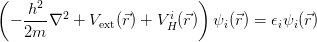
![( 2 )
− -h--∇2 + V [n(⃗r)] ϕ (⃗r) = ϵ ϕ (⃗r)
2m eff n n n
∑
n (⃗r) = ϕ ∗n(⃗r)ϕn(⃗r)
n,occ](thesis84x.png) | (2.28) (2.29) |
A common method used to calculate the exchange and correlation term (and that which is used in Chapter 3) is the local density approximation (LDA):
![∫
3
EXC [n ] = d rn(⃗r)ϵXC (n (⃗r))
where ϵXC(n) = ϵX(n) + ϵC(n)](thesis85x.png) | (2.30) |
An alternative method is the generalised gradient approximation (GGA):
![∫
EXC [n] = d3rn (⃗r)ϵXC(n(⃗r),∇n (⃗r))](thesis86x.png) | (2.31) |
Both the GGA and LDA have their strengths and weaknesses, e.g. with the LDA, the geometry of molecules on surfaces tends to be well-described, however their binding energies are underestimated. Similarly the GGA can yield improvements in the binding energies over LDA, but can overcorrect for the lattice constants in solids.
Further improvements can be made by including higher order gradient terms, however at the expense of higher computational demand. The Perdew-Burke-Ernzerhof formulation of the GGA [62] is used in Chapter 5 to optimise the different molecular conformations.
Some of the most drastic advances in recent years have been the development of DFT with van der Waals corrections included [63]. These come in various flavours [64–68], each with its own strengths and weaknesses, and some are advanced enough to be included in major commercial DFT codes such as VASP [69], however the open questions that remain promise to maintain the vibrancy this field has shown in recent years.
In order to solve the Kohn-Sham equations (Equation 2.28), they must be expanded in some basis set and solved as a linear eigenvalue problem, however there are several choices for the basis set: plane waves, local orbitals, or augmented functions.
In general, valence orbital wavefunctions tend to have many oscillations close to the atomic core, in order to maintain orthogonality with core states, however this introduces many Fourier components. A common method to alleviate this complexity is to replace them with a more simple pseudo-wavefunction which matches the real wavefunction beyond a specific cut-off radius, as can be seen in Figure 2.13, and can be represented by a small number of plane waves.
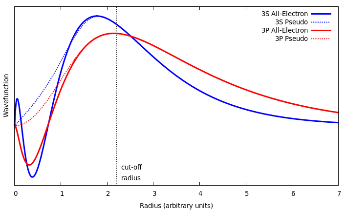
Similarly, the Coulomb potential wells centred on the ionic cores are very deep, and so it is common to use a smooth pseudopotential with the same scattering properties as the real potential. In this work, the augmented- plane-waves method is used with the projected augmented wave (PAW) pseudopotentials [70] included in the Vienna Ab initio Simulation Package (VASP).
The construction of accurate, transferable, and ultrasoft pseudopotentials could be the subject of an entire thesis in itself and so will not be described in detail here.
Since the Fermi level is the level of the highest occupied energy state of a
material, its position determines whether that material is an insulator or
conductor. If the Fermi level falls inside a gap in the band structure, that material
is an insulator. This means that the density of states smoothly goes to
zero before the band gap, and its  -integration does not cause problems
during calculation. For conductors however, the occupation at the Fermi
level is sharp, which makes integration and the use of plane-waves very
difficult.
-integration does not cause problems
during calculation. For conductors however, the occupation at the Fermi
level is sharp, which makes integration and the use of plane-waves very
difficult.
Increasing the number of k-points will cause the Fermi level to oscillate around its exact value, however by allowing k-points to be partially occupied (i.e. through smearing), a smaller number of k-points will yield an accurate band structure.
A symptom of this oscillation is the so-called “charge sloshing” where, for a small band-gap material, the electrons may transfer from a filled energy level to an unoccupied one during one iteration, however this switches the ordering of the levels, and the electrons “slosh” back in the next iteration. This can lead to calculations on small band-gap materials to converge slowly or never converge at all.
To solve this problem, the occupancies of the levels are “smeared out” using Fermi statistics, simulating an artificial temperature. In essence we are calculating the integral over the filled parts of the bands:
 | (2.32) |
 | (2.33) |
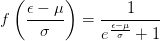 | (2.34) |
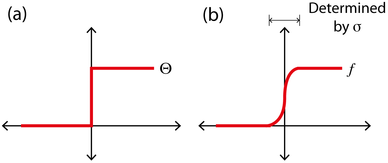
The method of Methfessel and Paxton solves this problem by expanding Θ in a complete orthonormal set of Hermite functions, of order N, for which N = 0 recovers the Gaussian approximation [72].
 | (2.35) |
The energy is then replaced by a generalised free energy functional F = E −∑ nkwkσS(fnk), however the entropy term ∑ nkwkσS(fnk) is very small for reasonable values of σ. The main drawbacks of the Methfessel and Paxton method are that it can introduce unphysical negative occupations, and increasing the order N introduces extra oscillations into the density of states, which can mask the real features.