2.1 Auger electron spectroscopy
Auger electron spectroscopy (AES) is a surface-sensitive and most importantly
material-sensitive technique based on the Auger effect, which allows the
characterisation of a surface’s cleanliness and make-up. The Auger effect was
discovered independently by Lise Meitner [51] and Pierre Auger [52] in the 1920s,
however it wasn’t until the 1950s that its value as an experimental technique was
realised.
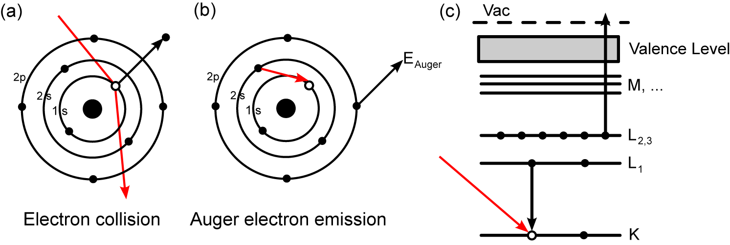
2.1.1 The Auger effect
The Auger effect describes the non-radiative emission of an electron after
a core vacancy is filled. A schematic of the Auger process is shown in
Figure 2.1.
A high-energy electron (or photon) collides with an atom, causing
the emission of a core electron (Figure 2.1a). The vacancy left behind is
then filled by an outer-shell electron (Figure 2.1b). The energy released
then stimulates the emission of an Auger electron, which can be detected
and analysed. The kinetic energy of the Auger electron is the difference
between the initial transition (L1 → K in Figure 2.1c) and the Auger
electron’s ionisation energy (L2,3). The Auger electron is defined by the
spectroscopic notation of the energy levels involved in its emission (KL1L2,3 in
Figure 2.1).
The K, L, M, etc. nomenclature used to describe the transitions is something
of a holdover from the early days of X-ray research. The Nobel laureate Charles
G. Barkla first noticed that some X-rays were able to penetrate thicker sheets of
metal than others. He began to characterise these differing penetration
“strengths” as “A” for more penetrating and “B” for less penetrating, however he
worried that further types of X-rays would be discovered, and so reclassified A as
K and B as L, to leave the labels A–J free. We now know that his K-type
rays were produced by the refilling of the innermost 1s shell in a manner
similar to that in Figure 2.1, and there can be no A–J transitions to
closer-bound orbitals, however the nomenclature has been kept for historical
reasons.
In this way, this terminology is commonly used in spectroscopic techniques
such as AES. An electronic orbital’s principal quantum number n is indicated
alphabetically by its letter, i.e. K (n = 1; 1s), L (n = 2; 2s, 2p), etc. The subscript
on L and higher gives a unique designation to each of the different orbitals which
may have the same n, but different l, s or j quantum numbers, i.e. L1 has
quantum numbers n = 2 and l = 0, and so corresponds to the 2s orbital; L2 is
2p(1∕2) with n = 2, l = 1, j =  and L3 is 2p(3∕2) with n = 2, l = 1, j =
  , and so
on in order of increasing energy. When a transition involves multiple orbitals it is
described by the orbitals’ spectroscopic notation, such as the KL1L2,3 transition
in Figure 2.1.
, and so
on in order of increasing energy. When a transition involves multiple orbitals it is
described by the orbitals’ spectroscopic notation, such as the KL1L2,3 transition
in Figure 2.1.
2.1.2 Auger electron spectroscopy
The energies of Auger transitions are specific to each element and its chemical
environment, so that its Auger spectrum acts as an elemental “fingerprint”, which
can be compared to a catalogue of known spectra. Each element typically has one
or more “characteristic peaks” which can be used to detect its presence in
complex spectra, e.g. when organic molecules are deposited on a surface, or when
testing a surface for possible contamination.
Due to the high linear background signal, the Auger spectrum is usually
represented as a differentiated spectrum, i.e.  vs. E. Due to the fact that the
differential of a peak (i.e. its slope) will be represented as first a negative and
then positive double peak, it is usual to refer only to the negative peak’s
position.
vs. E. Due to the fact that the
differential of a peak (i.e. its slope) will be represented as first a negative and
then positive double peak, it is usual to refer only to the negative peak’s
position.
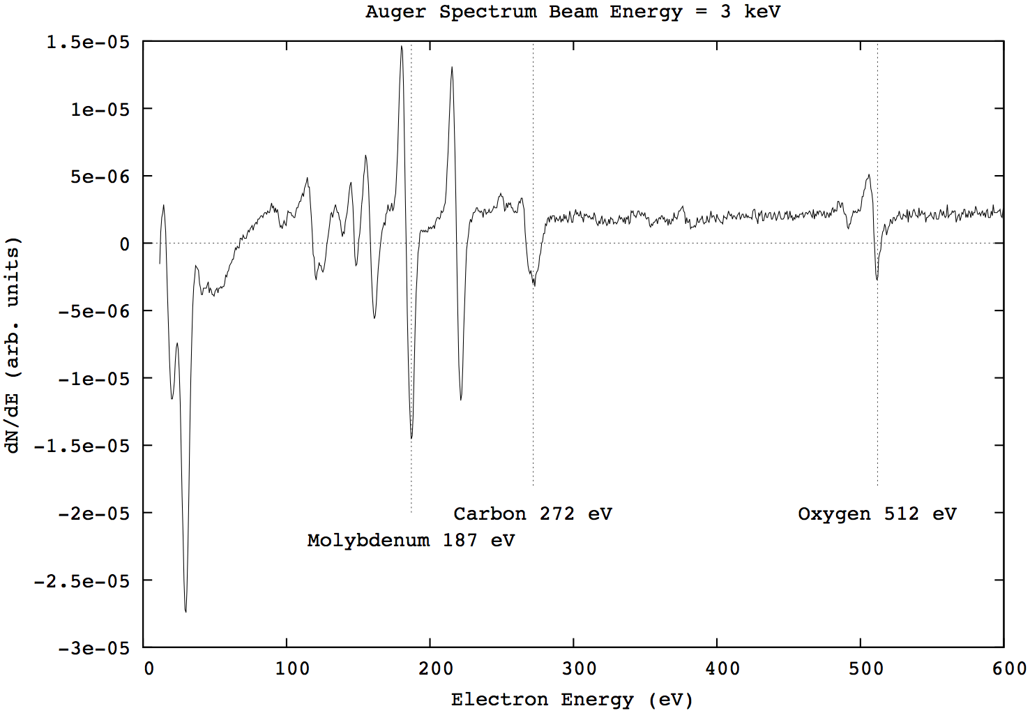
An example spectrum of a dirty Mo(110) sample is shown in Figure 2.2. The
characteristic peaks of molybdenum (187 eV), and the two main contaminants,
oxygen (512 eV) and carbon (272 eV), are highlighted.
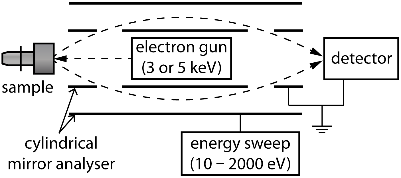
2.1.3 Auger electron spectroscopy set-up
Figure 2.3 shows the experimental set-up of the Auger electron spectroscopy
apparatus. 3–5 keV electrons are emitted by the electron gun and collide with the
sample. The resulting Auger electrons are passed through a cylindrical mirror
analyser (CMA).
The CMA consists of two concentric cylinders, the outer, which can have a
bias of -10 V to -2000 V placed upon it, and the inner, which is grounded.
Two apertures allow a narrow beam of Auger electrons to enter the space
between the two cylinders, where they are repelled by the outer bias. The
shape of the CMA is designed so that only those electrons with the same
energy as the outer bias can pass through both apertures and arrive at the
detector.
In this way the CMA selects the electrons according to their energy by
sweeping through energies from 10–2000 eV, however, partial sweeps can also
be used to more quickly screen samples, and to limit the time they are
subjected to high energy 3–5 keV electrons, which can damage surface
structures.