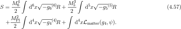
 -decoupling
limit of bi-gravity
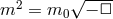
-decoupling
limit of bi-gravity
 )
)4 The Dvali–Gabadadze–Porrati Model
The idea behind the DGP model [209*, 208*, 207*] is to start with a four-dimensional braneworld in an infinite size-extra dimension. A priori gravity would then be fully five-dimensional, with respective Planck scale , but the matter fields localized on the brane could lead to an induced curvature term on the
brane with respective Planck scale
, but the matter fields localized on the brane could lead to an induced curvature term on the
brane with respective Planck scale  . See [22] for a potential embedding of this model within string
theory.
. See [22] for a potential embedding of this model within string
theory.
At small distances the induced curvature dominates and gravity behaves as in four dimensions, while at large distances the leakage of gravity within the extra dimension weakens the force of gravity. The DGP model is thus a model of modified gravity in the infrared, and as we shall see, the graviton effectively acquires a soft mass, or resonance.
4.1 Gravity induced on a brane
We start with the five-dimensional action for the DGP model [209, 208, 207] with a brane localized at
 ,
,
![∫ ( 3∘ ----- [√ --- 2 ]) S = d4x dy M-5- − (5)g (5)R + δ (y ) − gM-PlR [g ] + ℒm (g,ψi) , (4.1 ) 4 2](article401x.gif)
 represent matter field species confined to the brane with stress-energy tensor
  . This brane
is considered to be an orbifold brane enjoying a
. This brane
is considered to be an orbifold brane enjoying a  -orbifold symmetry (so that the physics at
  is
the mirror copy of that at
is
the mirror copy of that at  .) We choose the convention where we consider
  , reason
why we have a factor or
, reason
why we have a factor or  rather than
  if we had only consider one side of the brane, for
instance
if we had only consider one side of the brane, for
instance  .
.
The five-dimensional Einstein equation of motion are then given by
with The Israel matching condition on the brane [323] can be obtained by integrating this equation over

 and taking the limit
  , so that the jump in the extrinsic curvature across the brane
is related to the Einstein tensor and stress-energy tensor of the matter field confined on the
brane.
, so that the jump in the extrinsic curvature across the brane
is related to the Einstein tensor and stress-energy tensor of the matter field confined on the
brane.
4.1.1 Perturbations about flat spacetime
In DGP the four-dimensional graviton is effectively massive. To see this explicitly, we look at perturbations about flat spacetime
Since at this level we are dealing with five-dimensional GR, we are free to set the five-dimensional gauge of our choice and choose five-dimensional de Donder gauge (a discussion about the brane-bending mode will follow)

In this gauge the five-dimensional Einstein tensor is simply
where
 is the five-dimensional d’Alembertian and
  is the four-dimensional
one.
is the four-dimensional
one.
Since there is no source along the  or
or  directions (
 ), we can immediately
infer that
), we can immediately
infer that

 . We will see in Section 4.2 how to keep track of the brane-bending mode which is partly
encoded in
. We will see in Section 4.2 how to keep track of the brane-bending mode which is partly
encoded in  .
.
Using these relations in the five-dimensional de Donder gauge, we deduce the relation for the purely four-dimensional part of the metric perturbation,
Using these relations in the projected Einstein equation, we get where
![1- 3 [ 2] ( 2 ) 2 M 5 □ + ∂y (h μν − h ημν) = − δ(y ) 2Tμν + M Pl(□h μν − ∂μ∂νh ) , (4.10 )](article427x.gif)
 is the four-dimensional trace of the perturbations.
Solving this equation with the requirement that  as
as  , we infer the following profile
for the perturbations along the extra dimension
, we infer the following profile
for the perturbations along the extra dimension

 should really be thought in Fourier space, and
  is set from the boundary conditions
on the brane. Integrating the Einstein equation across the brane, from
is set from the boundary conditions
on the brane. Integrating the Einstein equation across the brane, from  to
to  , we get
yielding the modified linearized Einstein equation on the brane
where all the metric perturbations are the ones localized at
, we get
yielding the modified linearized Einstein equation on the brane
where all the metric perturbations are the ones localized at ![1-lim M 3[∂ h (x,y) − h(x, y)η ]𝜀 + M 2(□h (x,0) − ∂ ∂ h (x,0)) 2 𝜀→0 5 y μν μν− 𝜀 Pl μν μ ν = − 2Tμν(x), (4.12 )](article436x.gif)
![[ √ ---- ] M 2Pl (□h μν − ∂μ ∂νh) − m0 − □ (hμν − hη μν) = − 2T μν, (4.13 )](article437x.gif)
 and the constant mass scale
  is
given by
Interestingly, we see the special Fierz–Pauli combination
is
given by
Interestingly, we see the special Fierz–Pauli combination 
 appearing naturally
from the five-dimensional nature of the theory. At this level, this corresponds to a linearized
theory of massive gravity with a scale-dependent effective mass
appearing naturally
from the five-dimensional nature of the theory. At this level, this corresponds to a linearized
theory of massive gravity with a scale-dependent effective mass  , which
can be thought in Fourier space,
, which
can be thought in Fourier space,  . We could now follow the same procedure as
derived in Section 2.2.3 and obtain the expression for the sourced metric fluctuation on the brane
where
. We could now follow the same procedure as
derived in Section 2.2.3 and obtain the expression for the sourced metric fluctuation on the brane
where 
 is the trace of the four-dimensional stress-energy tensor localized on the brane. This
yields the following gravitational exchange amplitude between two conserved sources
is the trace of the four-dimensional stress-energy tensor localized on the brane. This
yields the following gravitational exchange amplitude between two conserved sources  and
and  ,
where the polarization tensor
,
where the polarization tensor 
 is the same as that given for Fierz–Pauli in (2.57*) in terms of
  .
In particular the polarization tensor includes the standard factor of
.
In particular the polarization tensor includes the standard factor of  as opposed to
  as would be the case in GR. This is again the manifestation of the vDVZ discontinuity which is
cured by the Vainshtein mechanism as for Fierz–Pauli massive gravity. See [165*] for the explicit
realization of the Vainshtein mechanism in DGP which is where it was first shown to work
explicitly.
as would be the case in GR. This is again the manifestation of the vDVZ discontinuity which is
cured by the Vainshtein mechanism as for Fierz–Pauli massive gravity. See [165*] for the explicit
realization of the Vainshtein mechanism in DGP which is where it was first shown to work
explicitly.
4.1.2 Spectral representation
In Fourier space the propagator for the graviton in DGP is given by
with the massive polarization tensor
 defined in (2.58*) and
which can be written in the Källén–Lehmann spectral representation as a sum of free propagators with
mass
defined in (2.58*) and
which can be written in the Källén–Lehmann spectral representation as a sum of free propagators with
mass 
 ,
with the spectral density
,
with the spectral density 
 which is represented in Figure 1*. As already emphasized, the graviton in DGP cannot be thought of a single
massive mode, but rather as a resonance picked about
which is represented in Figure 1*. As already emphasized, the graviton in DGP cannot be thought of a single
massive mode, but rather as a resonance picked about 
 .
.
We see that the spectral density is positive for any  , confirming the fact that about the normal
(flat) branch of DGP there is no ghost.
, confirming the fact that about the normal
(flat) branch of DGP there is no ghost.
Notice as well that in the massless limit  , we see appearing a representation of the Dirac delta
function,
, we see appearing a representation of the Dirac delta
function,

 which is the origin of the vDVZ discontinuity see Section 2.2.3.)
4.2 Brane-bending mode
Five-dimensional gauge-fixing
In Section 4.1.1 we have remained vague about the gauge-fixing and the implications for the brane position. The brane-bending mode is actually important to keep track of in DGP and we shall do that properly in what follows by keeping all the modes.
We work in the five-dimensional ADM split with the lapse  , the shift
 and the four-dimensional part of the metric,
  . The five-dimensional
Einstein–Hilbert term is then expressed as
. The five-dimensional
Einstein–Hilbert term is then expressed as
![(5) M-53√ --- ( 2 2) ℒ R = 4 − gN R [g] + [K ] − [K ] , (4.22 )](article468x.gif)
 and
and  is the extrinsic curvature
and
is the extrinsic curvature
and 
 is the covariant derivative with respect to
  .
.
First notice that the five-dimensional de Donder gauge choice (4.5*) can be made using the five-dimensional gauge fixing term
where we keep the same notation as previously,![3 ( )2 ℒ (5) = − M-5- ∂AhA − 1∂BhA (4.24 ) Gauge−Fixing 8 B 2 A 3 [( )2 = − M-5- ∂μhμ − 1∂νh + ∂yN ν − 1∂ νhyy (4.25 ) 8 ν 2 2 ( )2 ] μ 1- 1- + ∂μN + 2∂yhyy − 2 ∂yh ,](article474x.gif)
 is the four-dimensional trace.
After fixing the de Donder gauge (4.5*), we can make the addition gauge transformation
 , and remain in de Donder gauge provided
  satisfies linearly
  . This residual
gauge freedom can be used to further fix the gauge on the brane (see [389*] for more details, we only
summarize their derivation here).
. This residual
gauge freedom can be used to further fix the gauge on the brane (see [389*] for more details, we only
summarize their derivation here).
Four-dimensional Gauge-fixing
Keeping the brane at the fixed position  imposes
  since we need
  and
and  should be bounded as
  (the situation is slightly different in the self-accelerating branch and this
mode can lead to a ghost, see Section 4.4 as well as [361*, 98*]).
(the situation is slightly different in the self-accelerating branch and this
mode can lead to a ghost, see Section 4.4 as well as [361*, 98*]).
Using the bulk profile  and integrating over the extra dimension, we obtain
the contribution from the bulk on the brane (including the contribution from the gauge-fixing term) in
terms of the gauge invariant quantity
and integrating over the extra dimension, we obtain
the contribution from the bulk on the brane (including the contribution from the gauge-fixing term) in
terms of the gauge invariant quantity

![[ ] M 3 ∫ 1 √ ----( 1 ) 1 √ ----( 1 ) Sibnutelgkrated= --5- d4x − -&tidle;hμν − □ &tidle;hμν − -&tidle;h ημν + --hyy − □ &tidle;h − -hyy . 4 2 2 2 2](article486x.gif)
 to
to  imposing a
  -mirror symmetry at
  , rather than considering only one side of the
brane as in [389*]. Both conventions are perfectly reasonable.
, rather than considering only one side of the
brane as in [389*]. Both conventions are perfectly reasonable.
The integrated bulk action (4.27*) is invariant under the residual linearized gauge symmetry
which keeps both
 and
and  invariant. The residual gauge symmetry can be used to set the gauge on
the brane, and at this level from (4.27*) we can see that the most convenient gauge fixing term is [389*]
with again
invariant. The residual gauge symmetry can be used to set the gauge on
the brane, and at this level from (4.27*) we can see that the most convenient gauge fixing term is [389*]
with again 
 , so that the induced Lagrangian on the brane (including the contribution from
the residual gauge fixing term) is
Combining the five-dimensional action from the bulk (4.27*) with that on the boundary (4.31*) we end up
with the linearized action on the four-dimensional DGP brane [389*]
As shown earlier we recover the theory of a massive graviton in four dimensions, with a soft mass
, so that the induced Lagrangian on the brane (including the contribution from
the residual gauge fixing term) is
Combining the five-dimensional action from the bulk (4.27*) with that on the boundary (4.31*) we end up
with the linearized action on the four-dimensional DGP brane [389*]
As shown earlier we recover the theory of a massive graviton in four dimensions, with a soft mass
![∫ [ ( ) ] M P2l 4 1 μν 1 αμ 1 μ 2 μ Sboundary = --4- d x 2h □ (hμν − 2h ημν) − 2m0N μ ∂ αh − 2∂ h − m 0N μN . (4.31 )](article496x.gif)
![2 ∫ [ S(lin)= M-Pl d4x 1-hμν [□ − m √ − □-] (h − 1hη ) − m N μ∂ h (4.32 ) DGP 4 2 0 μν 2 μν 0 μ yy ] μ [√---- ] m0 √ ---- − m0N − □ + m0 N μ − -4-hyy − □(hyy − 2h ) .](article497x.gif)
 . This analysis has allowed us to keep track of the physical origin of all the modes
including the brane-bending mode which is especially relevant when deriving the decoupling limit as we
shall see below.
. This analysis has allowed us to keep track of the physical origin of all the modes
including the brane-bending mode which is especially relevant when deriving the decoupling limit as we
shall see below.
The kinetic mixing between these different modes can be diagonalized by performing the change of variables [389*]
so we see that the mode
 is directly related to
  . In the case of Section 4.1.1, we had set
  and the field
  is then related to the brane bending mode. In either case we see that the extrinsic
curvature
is then related to the brane bending mode. In either case we see that the extrinsic
curvature  carries part of this mode.
Omitting the mass terms and other relevant operators, the action is diagonalized in terms of the
different graviton modes at the linearized level  (which encodes the helicity-2 mode),
  (which is
part of the helicity-1 mode) and
(which is
part of the helicity-1 mode) and  (helicity-0 mode),
![∫ [ √---- ] S(lin) = 1- d4x 1h ′μν□ (h′ − 1h ′ημν) − N ′μ − □N ′+ 3π□ π . (4.36 ) DGP 4 2 μν 2 μ](article508x.gif)
Decoupling limit
We will be discussing the meaning of ‘decoupling limits’ in more depth in the context of multi-gravity and
ghost-free massive gravity in Section 8. The main idea behind the decoupling limit is to separate the
physics of the different modes. Here we are interested in following the interactions of the helicity-0 mode
without the complications from the standard helicity-2 interactions that already arise in GR. For this
purpose we can take the limit  while simultaneously sending
  while
keeping the scale
while
keeping the scale  fixed. This is the scale at which the first interactions arise in
DGP.
fixed. This is the scale at which the first interactions arise in
DGP.
In DGP the decoupling limit should be taken by considering the full five-dimensional theory, as was performed in [389*]. The four-dimensional Einstein–Hilbert term does not give to any operators before the Planck scale, so in order to look for the irrelevant operator that come at the lowest possible scale, it is sufficient to focus on the boundary term from the five-dimensional action. It includes operators of the form
with integer powers
 and
and  since we are dealing with interactions. The scale at
which such an operator arises is
and it is easy to see that the lowest possible scale is
since we are dealing with interactions. The scale at
which such an operator arises is
and it is easy to see that the lowest possible scale is 
 which arises for
  and
and
 , it is thus a cubic interaction in the helicity-0 mode
  which involves four derivatives. Since it is
only a cubic interaction, we can scan all the possible ways
which involves four derivatives. Since it is
only a cubic interaction, we can scan all the possible ways  enters at the cubic level in the
five-dimensional Einstein–Hilbert action. The relevant piece are the ones from the extrinsic curvature
in (4.22*), and in particular the combination
enters at the cubic level in the
five-dimensional Einstein–Hilbert action. The relevant piece are the ones from the extrinsic curvature
in (4.22*), and in particular the combination ![N ([K ]2 − [K2 ])](article521x.gif) , with
Integrating
, with
Integrating 
![m0M 2PlN ([K ]2 − [K2 ])](article523x.gif) along the extra dimension, we obtain the cubic contribution in
along the extra dimension, we obtain the cubic contribution in  on
the brane (using the relations (4.34*) and (4.35*))
So the decoupling limit of DGP arises at the scale
on
the brane (using the relations (4.34*) and (4.35*))
So the decoupling limit of DGP arises at the scale 
 and reduces to a cubic Galileon for the helicity-0
mode with no interactions for the helicity-2 and -1 modes,
and reduces to a cubic Galileon for the helicity-0
mode with no interactions for the helicity-2 and -1 modes,
4.3 Phenomenology of DGP
The phenomenology of DGP is extremely rich and has led to many developments. In what follows we review one of the most important implications of the DGP for cosmology which the existence of self-accelerating solutions. The cosmology and phenomenology of DGP was first derived in [159*, 163*] (see also [388*, 385*, 387*, 386*]).
4.3.1 Friedmann equation in de Sitter
To get some intuition on how cosmology gets modified in DGP, we first look at de Sitter-like solutions and then infer the full Friedmann equation in a FLRW-geometry. We thus start with five-dimensional Minkowski in de Sitter slicing (this can be easily generalized to FLRW-slicing),
where
 is the four-dimensional de Sitter metric with constant Hubble parameter
  ,
,
 , and the scale factor is given by
  . The metric (4.43*) is
indeed Minkowski in de Sitter slicing if the warp factor
. The metric (4.43*) is
indeed Minkowski in de Sitter slicing if the warp factor  is given by
and the mod
is given by
and the mod 
 has be imposed by the
  -orbifold symmetry. As we shall see the branch
  corresponds to the self-accelerating branch of DGP and
  is the stable, normal branch of
DGP.
is the stable, normal branch of
DGP.
We can now derive the Friedmann equation on the brane by integrating over the  -component of the
Einstein equation (4.2*) with the source (4.3*) and consider some energy density
-component of the
Einstein equation (4.2*) with the source (4.3*) and consider some energy density  . The
four-dimensional Einstein tensor gives the standard contribution
. The
four-dimensional Einstein tensor gives the standard contribution  on the brane and so we
obtain the modified Friedmann equation
on the brane and so we
obtain the modified Friedmann equation
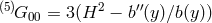
![M 3[ ∫ 𝜀 ] ---5 lim (5)G00 dy + 3M 2PlH2 = ρ, (4.45 ) 2 𝜀→0 − 𝜀](article542x.gif)
 , so
leading to the modified Friedmann equation,
where the five-dimensional nature of the theory is encoded in the new term
, so
leading to the modified Friedmann equation,
where the five-dimensional nature of the theory is encoded in the new term 

 (this new
contribution can be seen to arise from the helicity-0 mode of the graviton and could have been derived using
the decoupling limit of DGP.)
(this new
contribution can be seen to arise from the helicity-0 mode of the graviton and could have been derived using
the decoupling limit of DGP.)
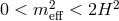
For reasons which will become clear in what follows, the choice  corresponds to the stable
branch of DGP while the other choice
corresponds to the stable
branch of DGP while the other choice  corresponds to the self-accelerating branch of DGP. As is
already clear from the higher-dimensional perspective, when
corresponds to the self-accelerating branch of DGP. As is
already clear from the higher-dimensional perspective, when  , the warp factor grows in the bulk
(unless we think of the junction conditions the other way around), which is already signaling towards a
pathology for that branch of solution.
, the warp factor grows in the bulk
(unless we think of the junction conditions the other way around), which is already signaling towards a
pathology for that branch of solution.
4.3.2 General Friedmann equation
This modified Friedmann equation has been derived assuming a constant  , which is only consistent if
the energy density is constant (i.e., a cosmological constant). We can now derive the generalization of this
Friedmann equation for non-constant
, which is only consistent if
the energy density is constant (i.e., a cosmological constant). We can now derive the generalization of this
Friedmann equation for non-constant  . This amounts to account for
  and other derivative
corrections which might have been omitted in deriving this equation by assuming that
and other derivative
corrections which might have been omitted in deriving this equation by assuming that  was
constant. But the Friedmann equation corresponds to the Hamiltonian constraint equation
and higher derivatives (e.g.,
was
constant. But the Friedmann equation corresponds to the Hamiltonian constraint equation
and higher derivatives (e.g.,  and higher derivatives of
  ) would imply that this
equation is no longer a constraint and this loss of constraint would imply that the theory admits a
new degree of freedom about generic backgrounds namely the BD ghost (see the discussion of
Section 7).
) would imply that this
equation is no longer a constraint and this loss of constraint would imply that the theory admits a
new degree of freedom about generic backgrounds namely the BD ghost (see the discussion of
Section 7).
However, in DGP we know that the BD ghost is absent (this is ensured by the five-dimensional nature of
the theory, in five dimensions we start with five dofs, and there is thus no sixth BD mode). So
the Friedmann equation cannot include any derivatives of  , and the Friedmann equation
obtained assuming a constant
, and the Friedmann equation
obtained assuming a constant  is actually exact in FLRW even if
  is not constant. So the
constraint (4.47*) is the exact Friedmann equation in DGP for any energy density
is not constant. So the
constraint (4.47*) is the exact Friedmann equation in DGP for any energy density  on the
brane.
on the
brane.
The same trick can be used for massive gravity and bi-gravity and the Friedmann equations (12.51*), (12.52*) and (12.54*) are indeed free of any derivatives of the Hubble parameter.
4.3.3 Observational viability of DGP
Independently of the ghost issue in the self-accelerating branch of the model, there has been a vast amount of investigation on the observational viability of both the self-accelerating branch and the normal (stable) branch of DGP. First because many of these observations can apply equally well to the stable branch of DGP (modulo a minus sign in some of the cases), and second and foremost because DGP represents an excellent archetype in which ideas of modified gravity can be tested.
Observational tests of DGP fall into the following two main categories:
- Tests of the Friedmann equation. This test was performed mainly using Supernovae, but
also using Baryonic Acoustic Oscillations and the CMB so as to fix the background history of the
Universe [162, 217, 221, 286, 391, 23, 405, 481, 304, 382, 462]. Current observations seem
to slightly disfavor the additional
 term in the Friedmann equation of DGP, even in the
normal branch where the late-time acceleration of the Universe is due to a cosmological constant
as in
term in the Friedmann equation of DGP, even in the
normal branch where the late-time acceleration of the Universe is due to a cosmological constant
as in  CDM. These put bounds on the graviton mass in DGP to the order of
  ,
where
,
where  is the Hubble parameter today (see Ref. [492] for the latest bounds at the time
of writing, including data from Planck). Effectively this means that in order for DGP to be
consistent with observations, the graviton mass can have no effect on the late-time acceleration
of the Universe.
is the Hubble parameter today (see Ref. [492] for the latest bounds at the time
of writing, including data from Planck). Effectively this means that in order for DGP to be
consistent with observations, the graviton mass can have no effect on the late-time acceleration
of the Universe.
- Tests of an extra fifth force, either within the solar system, or during structure formation
(see for instance [362, 260, 452, 451, 222, 482] Refs. [453, 337, 442] for N-body simulations
as well as Ref. [17, 441] using weak lensing).
Evading fifth force experiments will be discussed in more detail within the context of the Vainshtein mechanism in Section 10.1 and thereafter, and we save the discussion to that section. See Refs. [388*, 385, 387, 386*, 444] for a five-dimensional study dedicated to DGP. The study of cosmological perturbations within the context of DGP was also performed in depth for instance in [367, 92].
4.4 Self-acceleration branch
The cosmology of DGP has led to a major conceptual breakthrough, namely the realization that the
Universe could be ‘self-accelerating’. This occurs when choosing the  branch of DGP, the
Friedmann equation in the vacuum reduces to [159*, 163*]
branch of DGP, the
Friedmann equation in the vacuum reduces to [159*, 163*]

 in the absence of any cosmological constant nor
vacuum energy. In itself this would not solve the old cosmological constant problem as the
vacuum energy ought to be set to zero on its own, but it can lead to a model of ‘dark gravity’
where the amount of acceleration is governed by the scale
in the absence of any cosmological constant nor
vacuum energy. In itself this would not solve the old cosmological constant problem as the
vacuum energy ought to be set to zero on its own, but it can lead to a model of ‘dark gravity’
where the amount of acceleration is governed by the scale  which is stable against quantum
corrections.
which is stable against quantum
corrections.
This realization has opened a new field of study in its own right. It is beyond the scope of this review on massive gravity to summarize all the interesting developments that arose in the past decade and we simply focus on a few elements namely the presence of a ghost in this self-accelerating branch as well as a few cosmological observations.
Ghost
The existence of a ghost on the self-accelerating branch of DGP was first pointed out in the decoupling limit [389*, 411*], where the helicity-0 mode of the graviton is shown to enter with the wrong sign kinetic in this branch of solutions. We emphasize that the issue of the ghost in the self-accelerating branch of DGP is completely unrelated to the sixth BD ghost on some theories of massive gravity. In DGP there are five dofs one of which is a ghost. The analysis was then generalized in the fully fledged five-dimensional theory by K. Koyama in [360*] (see also [263, 361] and [98*]).
When perturbing about Minkowski, it was shown that the graviton has an effective mass
 . When perturbing on top of the self-accelerating solution a similar analysis can be
performed and one can show that in the vacuum the graviton has an effective mass at precisely
the Higuchi-bound,
. When perturbing on top of the self-accelerating solution a similar analysis can be
performed and one can show that in the vacuum the graviton has an effective mass at precisely
the Higuchi-bound,  (see Ref. [307*]). When matter or a cosmological constant
is included on the brane, the graviton mass shifts either inside the forbidden Higuchi-region
(see Ref. [307*]). When matter or a cosmological constant
is included on the brane, the graviton mass shifts either inside the forbidden Higuchi-region
 , or outside
  . We summarize the three case scenario following [360, 98]
- In [307*] it was shown that when the effective mass is within the forbidden Higuchi-region, the helicity-0 mode of graviton has the wrong sign kinetic term and is a ghost.
- Outside this forbidden region, when
 , the zero-mode of the graviton is healthy but
there exists a new normalizable brane-bending mode in the self-accelerating branch8
which is a genuine degree of freedom. For
, the zero-mode of the graviton is healthy but
there exists a new normalizable brane-bending mode in the self-accelerating branch8
which is a genuine degree of freedom. For  the brane-bending mode was shown to
be a ghost.
the brane-bending mode was shown to
be a ghost.
- Finally, at the critical mass
 (which happens when no matter nor cosmological
constant is present on the brane), the brane-bending mode takes the role of the helicity-0 mode
of the graviton, so that the theory graviton still has five degrees of freedom, and this mode was
shown to be a ghost as well.
(which happens when no matter nor cosmological
constant is present on the brane), the brane-bending mode takes the role of the helicity-0 mode
of the graviton, so that the theory graviton still has five degrees of freedom, and this mode was
shown to be a ghost as well.
In summary, independently of the matter content of the brane, so long as the graviton is massive  ,
the self-accelerating branch of DGP exhibits a ghost. See also [210] for an exact non-perturbative argument
studying domain walls in DGP. In the self-accelerating branch of DGP domain walls bear a negative
gravitational mass. This non-perturbative solution can also be used as an argument for the instability of
that branch.
,
the self-accelerating branch of DGP exhibits a ghost. See also [210] for an exact non-perturbative argument
studying domain walls in DGP. In the self-accelerating branch of DGP domain walls bear a negative
gravitational mass. This non-perturbative solution can also be used as an argument for the instability of
that branch.
Evading the ghost?
Different ways to remove the ghosts were discussed for instance in [325] where a second brane was included. In this scenario it was then shown that the graviton could be made stable but at the cost of including a new spin-0 mode (that appears as the mode describing the distance between the branes).
Alternatively it was pointed out in [233] that if the sign of the extrinsic curvature was flipped, the self-accelerating solution on the brane would be stable.
Finally, a stable self-acceleration was also shown to occur in the massless case  by relying on
Gauss–Bonnet terms in the bulk and a self-source AdS5 solution [156]. The five-dimensional theory is then
similar as that of DGP (4.1*) but with the addition of a five-dimensional Gauss–Bonnet term
by relying on
Gauss–Bonnet terms in the bulk and a self-source AdS5 solution [156]. The five-dimensional theory is then
similar as that of DGP (4.1*) but with the addition of a five-dimensional Gauss–Bonnet term  in the
bulk and the wrong sign five-dimensional Einstein–Hilbert term,
in the
bulk and the wrong sign five-dimensional Einstein–Hilbert term,
![[ ∫ ∘ -----( M 3 M 3ℓ2 ) S = d5x − (5)g − --5(5)R [(5)g] − --5--(5)ℛ2GB [(5)g] (4.49 ) 4 4 [ 2 ] ] + δ(y) √ − g-M-PlR + ℒ (g,ψ ) . 2 m i](article578x.gif)
 is related to this AdS
length scale, and the self-accelerating branch admits a stable (ghost-free) de Sitter solution with
is related to this AdS
length scale, and the self-accelerating branch admits a stable (ghost-free) de Sitter solution with
 .
.
We do not discuss this model any further in what follows since the graviton admits a zero (massless) mode. It is feasible that this model can be understood as a bi-gravity theory where the massive mode is a resonance. It would also be interesting to see how this model fits in with the Galileon theories [412*] which admit stable self-accelerating solution.
In what follows, we go back to the standard DGP model be it the self-accelerating branch ( ) or
the normal branch (
) or
the normal branch ( ).
).
4.5 Degravitation
One of the main motivations behind modifying gravity in the infrared is to tackle the old cosmological constant problem. The idea behind ‘degravitation’ [211*, 212*, 26*, 216*] is if gravity is modified in the IR, then a cosmological constant (or the vacuum energy) could have a smaller impact on the geometry. In these models, we would live with a large vacuum energy (be it at the TeV scale or at the Planck scale) but only observe a small amount of late-acceleration due to the modification of gravity. In order for a theory of modified gravity to potentially tackle the old cosmological constant problem via degravitation it needs to have the two following properties:
- 1.
- First, gravity must be weaker in the infrared and effectively massive [216*] so that the effect of IR sources can be degravitated.
- 2.
- Second, there must exist some (nearly) static attractor solutions towards which the system can evolve at late-time for arbitrary value of the vacuum energy or cosmological constant.
Flat solution with a cosmological constant
The first requirement is present in DGP, but as was shown in [216*] in DGP gravity is not ‘sufficiently weak’ in the IR to allow degravitation solutions. Nevertheless, it was shown in [164] that the normal branch of DGP satisfies the second requirement for any negative value of the cosmological constant. In these solutions the five-dimensional spacetime is not Lorentz invariant, but in a way which would not (at this background level) be observed when confined on the four-dimensional brane.
For positive values of the cosmological constant, DGP does not admit a (nearly) static solution. This can be understood at the level of the decoupling limit using the arguments of [216*] and generalized for other mass operators.
Inspired by the form of the graviton in DGP,  , we can generalize the form of the
graviton mass to
, we can generalize the form of the
graviton mass to

 a positive dimensionless constant.
  corresponds to a modification of the kinetic term. As
shown in [153*], any such modification leads to ghosts, so we do not consider this case here.
corresponds to a modification of the kinetic term. As
shown in [153*], any such modification leads to ghosts, so we do not consider this case here.  corresponds to a UV modification of gravity, and so we focus on
  .
.
In the decoupling limit the helicity-2 decouples from the helicity-0 mode which behaves (symbolically) as follows [216*]
where
 is the trace of the stress-energy tensor of external matter fields. At the linearized level, matter
couples to the metric
is the trace of the stress-energy tensor of external matter fields. At the linearized level, matter
couples to the metric  . We now check under which conditions we can still
recover a nearly static metric in the presence of a cosmological constant
. We now check under which conditions we can still
recover a nearly static metric in the presence of a cosmological constant  . In the linearized
limit of GR this leads to the profile for the helicity-2 mode (which in that case corresponds to a linearized
de Sitter solution)
One way we can obtain a static solution in this extended theory of massive gravity at the linear level is by
ensuring that the solution for
. In the linearized
limit of GR this leads to the profile for the helicity-2 mode (which in that case corresponds to a linearized
de Sitter solution)
One way we can obtain a static solution in this extended theory of massive gravity at the linear level is by
ensuring that the solution for 
 cancels out that of
  so that the metric
  remains flat.
 is actually the solution of (4.51*) when only the term
  contributes and all the
other operators vanish for
contributes and all the
other operators vanish for  . This is the case if
  as shown in [216*]. This explains why in
the case of DGP which corresponds to border line scenario
as shown in [216*]. This explains why in
the case of DGP which corresponds to border line scenario  , one can never fully degravitate a
cosmological constant.
, one can never fully degravitate a
cosmological constant.
Extensions
This realization has motivated the search for theories of massive gravity with  , and especially
the extension of DGP to higher dimensions where the parameter
, and especially
the extension of DGP to higher dimensions where the parameter  can get as close to zero as
required. This is the main motivation behind higher dimensional DGP [359, 240*] and cascading
gravity [135*, 148*, 132*, 149*] as we review in what follows. (In [433] it was also shown how a
regularized version of higher dimensional DGP could be free of the strong coupling and ghost
issues).
can get as close to zero as
required. This is the main motivation behind higher dimensional DGP [359, 240*] and cascading
gravity [135*, 148*, 132*, 149*] as we review in what follows. (In [433] it was also shown how a
regularized version of higher dimensional DGP could be free of the strong coupling and ghost
issues).
Note that  corresponds to a hard mass gravity. Within the context of DGP, such a model with
an ‘auxiliary’ extra dimension was proposed in [235, 133*] where we consider a finite-size large extra
dimension which breaks five-dimensional Lorentz invariance. The five-dimensional action is
motivated by the five-dimensional gravity with scalar curvature in the ADM decomposition
corresponds to a hard mass gravity. Within the context of DGP, such a model with
an ‘auxiliary’ extra dimension was proposed in [235, 133*] where we consider a finite-size large extra
dimension which breaks five-dimensional Lorentz invariance. The five-dimensional action is
motivated by the five-dimensional gravity with scalar curvature in the ADM decomposition
![(5)R = R [g] + [K ]2 − [K2 ]](article605x.gif) , but discarding the contribution from the four-dimensional curvature
, but discarding the contribution from the four-dimensional curvature
![R [g]](article606x.gif) . Similarly as in DGP, the four-dimensional curvature still appears induced on the brane
. Similarly as in DGP, the four-dimensional curvature still appears induced on the brane
![M 2Pl∫ ℓ ∫ 4 √ ---( ( 2 2 ) ) S = ---- dy d x − g m0 [K ] − [K ] + δ(y)R[g] , (4.53 ) 2 0](article607x.gif)
 is the size of the auxiliary extra dimension and
  is a four-dimensional metric and we set the
lapse to one (this shift can be kept and will contribute to the four-dimensional Stückelberg field which
restores four-dimensional invariance, but at this level it is easier to work in the gauge where
the shift is set to zero and reintroduce the Stückelberg fields directly in four dimensions).
Imposing the Dirichlet conditions
is a four-dimensional metric and we set the
lapse to one (this shift can be kept and will contribute to the four-dimensional Stückelberg field which
restores four-dimensional invariance, but at this level it is easier to work in the gauge where
the shift is set to zero and reintroduce the Stückelberg fields directly in four dimensions).
Imposing the Dirichlet conditions  , we are left with a theory of massive
gravity at
, we are left with a theory of massive
gravity at  , with reference metric
  and hard mass
  . Here again the special
structure
. Here again the special
structure ![([K ]2 − [K2 ])](article614x.gif) inherited (or rather inspired) from five-dimensional gravity ensures the
Fierz–Pauli structure and the absence of ghost at the linearized level. Up to cubic order in
perturbations it was shown in [138*] that the theory is free of ghost and its decoupling limit is that of a
Galileon.
inherited (or rather inspired) from five-dimensional gravity ensures the
Fierz–Pauli structure and the absence of ghost at the linearized level. Up to cubic order in
perturbations it was shown in [138*] that the theory is free of ghost and its decoupling limit is that of a
Galileon.
Furthermore, it was shown in [133] that it satisfies both requirements presented above to potentially help degravitating a cosmological constant. Unfortunately at higher orders this model is plagued with the BD ghost [291] unless the boundary conditions are chosen appropriately [59]. For this reason we will not review this model any further in what follows and focus instead on the ghost-free theory of massive gravity derived in [137*, 144*]
4.5.1 Cascading gravity
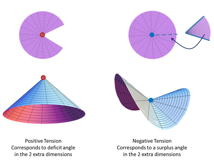
Deficit angle
It is well known that a tension on a cosmic string does not cause the cosmic strong to inflate but rather creates a deficit angle in the two spatial dimensions orthogonal to the string. Similarly, if we consider a four-dimensional brane embedded in six-dimensional gravity, then a tension on the brane leads to the following flat geometry
where the two extra dimensions are expressed in polar coordinates
 and
and  is a constant which
parameterize the deficit angle in this canonical geometry. This deficit angle is related to the tension
on the brane
is a constant which
parameterize the deficit angle in this canonical geometry. This deficit angle is related to the tension
on the brane  and the six-dimensional Planck scale (assuming six-dimensional gravity)
For a positive tension
and the six-dimensional Planck scale (assuming six-dimensional gravity)
For a positive tension 
 , this creates a positive deficit angle and since
  cannot be larger than
 , the maximal tension on the brane is
  . For a negative tension, on the other hand, there is no such
bound as it creates a surplus of angle, see Figure 2*.
. For a negative tension, on the other hand, there is no such
bound as it creates a surplus of angle, see Figure 2*.
This interesting feature has lead to many potential ways to tackle the cosmological constant by considering
our Universe to live in a  -dimensional brane embedded in two or more large extra dimensions. (See
Refs. [4, 3, 408, 414, 80, 470, 458, 459, 86, 82, 247, 333, 471, 81, 426, 409, 373, 85, 460, 155] for the
supersymmetric large-extra-dimension scenario as an alternative way to tackle the cosmological constant
problem). Extending the DGP to more than one extra dimension could thus provide a natural way to tackle
the cosmological constant problem.
-dimensional brane embedded in two or more large extra dimensions. (See
Refs. [4, 3, 408, 414, 80, 470, 458, 459, 86, 82, 247, 333, 471, 81, 426, 409, 373, 85, 460, 155] for the
supersymmetric large-extra-dimension scenario as an alternative way to tackle the cosmological constant
problem). Extending the DGP to more than one extra dimension could thus provide a natural way to tackle
the cosmological constant problem.
Spectral representation
Furthermore in  -extra dimensions the gravitational potential is diluted as
  . If the
propagator has a Källén–Lehmann spectral representation with spectral density
. If the
propagator has a Källén–Lehmann spectral representation with spectral density  , the Newtonian
potential has the following spectral representation
, the Newtonian
potential has the following spectral representation

 which implies
  in the IR as depicted in Figure 1*.
Working back in terms of the spectral representation of the propagator as given in (4.19*), this means
that the propagator goes to  in the IR as
  when
when  (as we know from DGP), while it
goes to a constant for
(as we know from DGP), while it
goes to a constant for  . So for more than one extra dimension, the theory tends towards that of a
hard mass graviton in the far IR, which corresponds to
. So for more than one extra dimension, the theory tends towards that of a
hard mass graviton in the far IR, which corresponds to  in the parametrization of (4.50*). Following
the arguments of [216*] such a theory should thus be a good candidate to tackle the cosmological constant
problem.
in the parametrization of (4.50*). Following
the arguments of [216*] such a theory should thus be a good candidate to tackle the cosmological constant
problem.
A brane on a brane
Both the spectral representation and the fact that codimension-two (and higher) branes can accommodate for a cosmological constant while remaining flat has made the field of higher-codimension branes particularly interesting.
However, as shown in [240*] and [135*, 148*, 132, 149*], the straightforward extension of DGP to two large extra dimensions leads to ghost issues (sixth mode with the wrong sign kinetic term, see also [290, 70]) as well as divergences problems (see Refs. [256, 131, 130, 423, 422, 355, 83]).
To avoid these issues, one can consider simply applying the DGP procedure step by step and
consider a  -dimensional DGP brane embedded in six dimension. Our Universe would
then be on a
-dimensional DGP brane embedded in six dimension. Our Universe would
then be on a  -dimensional DGP brane embedded in the
  one, (note we only
consider one side of the brane here which explains the factor of 2 difference compared with (4.1*))
one, (note we only
consider one side of the brane here which explains the factor of 2 difference compared with (4.1*))
 which characterizes the scale at which one crosses
from the four-dimensional to the five-dimensional regime, and
which characterizes the scale at which one crosses
from the four-dimensional to the five-dimensional regime, and  yielding the crossing from a
five-dimensional to a six-dimensional behavior. Of course we could also have a simultaneous crossing if
yielding the crossing from a
five-dimensional to a six-dimensional behavior. Of course we could also have a simultaneous crossing if
 . In what follows we focus on the case where
  .
.
Performing the same linearized analysis as in Section 4.1.1 we can see that the four-dimensional theory of gravity is effectively massive with the soft mass in Fourier space
We see that the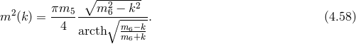
 -dimensional brane plays the role of a regulator (a divergence occurs in the limit
 ).
).
In this six-dimensional model, there are effectively two new scalar degrees of freedom (arising from the extra dimensions). We can ensure that both of them have the correct sign kinetic term by
- Either smoothing out the brane [240, 148] (this means that one should really consider a
six-dimensional curvature on both the smoothed
 and on the
  -dimensional branes,
which is something one would naturally expect9).
-dimensional branes,
which is something one would naturally expect9).
- Or by including some tension on the
 brane (which is also something natural since the
setup is designed to degravitate a large cosmological constant on that brane). This was shown
to be ghost free in the decoupling limit in [135] and in the full theory in [150].
brane (which is also something natural since the
setup is designed to degravitate a large cosmological constant on that brane). This was shown
to be ghost free in the decoupling limit in [135] and in the full theory in [150].
As already mentioned in two large extra dimensional models there is to be a maximal value of the cosmological constant that can be considered which is related to the six-dimensional Planck scale. Since that scale is in turn related to the effective mass of the graviton and since observations set that scale to be relatively small, the model can only take care of a relatively small cosmological constant. Nevertheless, it still provides a proof of principle on how to evade Weinberg’s no-go theorem [484*].
The extension of cascading gravity to more than two extra dimensions was considered in [149*]. It was
shown in that case how the  brane remains flat for arbitrary values of the cosmological constant on
that brane (within the regime of validity of the weak-field approximation). See Figure 3* for a picture on
how the scalar potential adapts itself along the extra dimensions to accommodate for a cosmological
constant on the brane.
brane remains flat for arbitrary values of the cosmological constant on
that brane (within the regime of validity of the weak-field approximation). See Figure 3* for a picture on
how the scalar potential adapts itself along the extra dimensions to accommodate for a cosmological
constant on the brane.
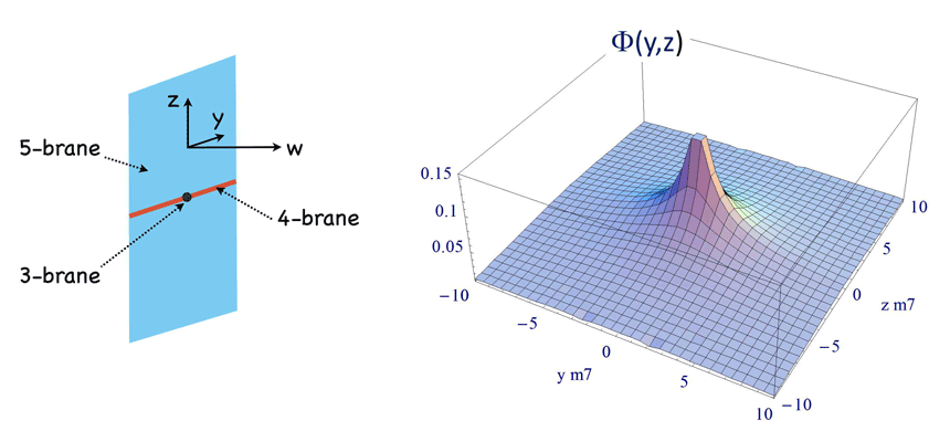
 on
the
on
the  -dimensional brane in a 7-dimensional cascading gravity scenario with tension on the
 -dimensional brane located at
  , in the case where
  .
.
 and
and  represent the two extra dimensions on the
  -dimensional brane. Image
reproduced with permission from [149], copyright APS.
-dimensional brane. Image
reproduced with permission from [149], copyright APS.
 |
 |
 |
Living Rev. Relativity, 17 (2014), 7, doi:10.12942/lrr-2014-7, URL (accessed <date>): http://www.livingreviews.org/lrr-2014-7.
 This work is licensed under a Creative Commons License.
© The author(s), except where otherwise noted.
This work is licensed under a Creative Commons License.
© The author(s), except where otherwise noted.