Research interest: Foams, Packing problems and Soft Matter
You might start your morning by washing your hair with shampoo or shaving yourself with shaving cream.
Then during the day, you maybe refuel yourself with a nice cup of cappuccino and clean the cup afterward with detergents.
If you work as a fire fighter, professionally or voluntarily, you might consider fire-fighting foam as one of your strongest allies.
And at the end of an exhausting day, you might relax with a pint of Guinness (or any other inferior beer).
These are only a few examples from our everyday life, where foam is of paramount importance.
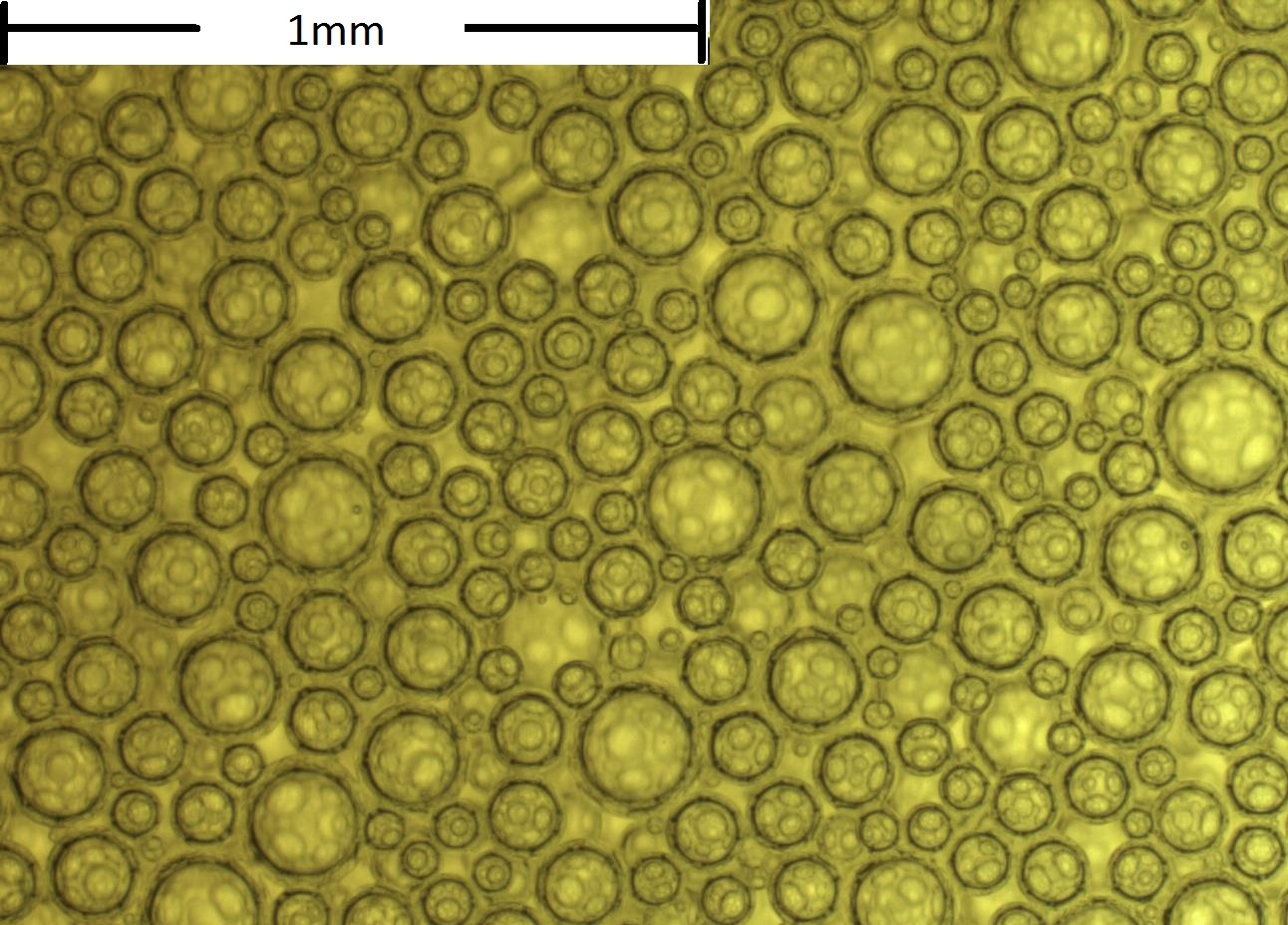
Microscopic picture of a Guinness foam. The smooth foam is due to the small bubbles of nitrogen gas.
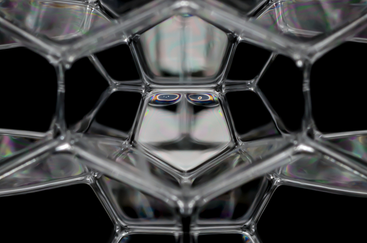
Photography of a dry foam by Kym Cox. More images of foams and bubbles can be found on her website.
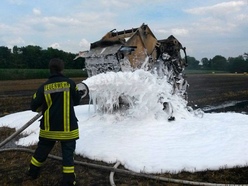
Fire brigade (from Datteln) extinguish a burning hay baler with foam. Thank you Marie!
But the real beauty of foams is the ability to transfer its abstract features to analogous complex systems.
People jammed into over-crowded pubs, huddling Emperor penguins, cells in biological tissues, and platelets in blood vessels are just some examples on different length scales and in different contexts of such complex systems.
Foams, i.e. dense packings of gas bubbles in a liquid, serve as a good model system for these packing problems of soft objects because bubbles are well approximated as deformable, frictionless particles.
Jamming of soft particles can have dramatic implications, as in the case of an evacuation of a building in emergency, or the formation of a blood clot.
Thus, while studying foams seems to be a very niche field, it is much more than just a fun research area.
It is a laboratory model for other systems that comes without the complexity of the research field it is supposed to simulate.
Systems of dry foam (up to 5% liquid fraction) have been investigated for a couple of lustrums and their governing laws are well understood (see also Plateau's laws).
Current research focuses more on wet foam up to the jamming point with a liquid fraction of 36% in three dimensions and 16% in two dimensions.
At these limits the densely packed bubbles have spherical shape and thus wet foam is sometimes modeled as a dense packing of overlapping spheres [Durian96].
While this works for a first approximation and we will use it as such to investigate columnar packings, we will also show the limits of this approximation in our 2D foam simulations.
Three areas of my research related to foams, packing problems, and soft matter are covered below:
Columnar soft sphere packings:
Here I show you some packings obtained from simulations of soft spheres confined in cylindrical confinements and where these packings appear in science and nature.
A phase diagram of all structures without internal spheres is presented, as well as some stability investigations.
2D foam simulations:
Results from an ideal 2D foam simulation, called Plat, is compared to the popular bubble model, which is used to simulate wet foam.
However, here I show some of the limits of this simulation method and propose a new model, based on the Morse-Witten theory.
Ordered packings of spheres in cylindrical confinements have been studied for over a century, initially applied to biological systems, such as seeds around a stem.
But in recent years such columnar packings have been discovered in various research fields on various length scales, ranging from macroscopic systems such as foams [Tobin11] over micro-rods to the nanoscale, where those structures are used to create rods and fibers [Wu16, Troche05].
The last two are probably the most prestigious applications with huge potential as we will see.
A \( (3, {\bf{2}}, 1) \) line-slip packing in a columnar foam. More details are in the section below.
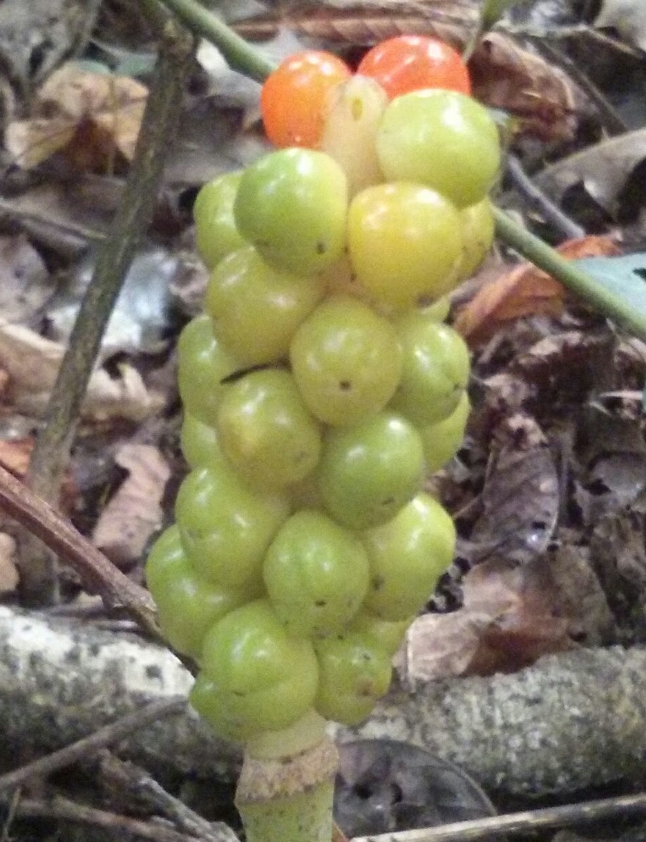
A \( (3, {\bf{2}}, 1) \) line-slip packing of seeds around a plant. I spotted this arum maculatum plant in Bushy Park, Dublin.
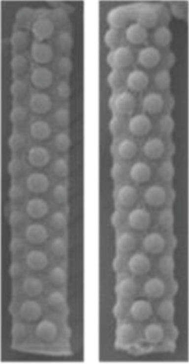
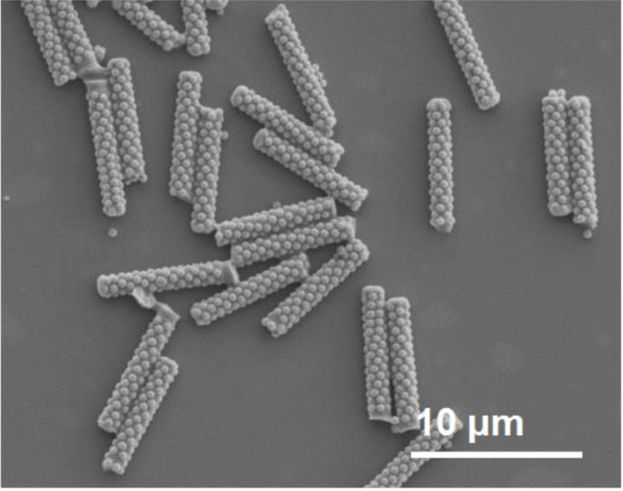
Columnar packings of silica particles on the surface of a cylinder on the micron scale. The structure alters physical properties of the cylinder.
Such packings can be used to manufacture micro-rods for novel materials such as liquid crystals [Wu16].
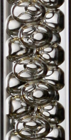
Columnar packings can easily be created in a forced drainage experiment by a foam column inside a tube (image on the far left).
The control parameters in such an experiment are then liquid fraction and bubble size.
In nature these sphere arrangements can be found in almost every park (at least here on the island of Ireland).
While strolling through Bushy Park in Dublin last year, the arum maculatum plant (see 2nd pic from the left) fell into my view at every corner.
I guess if you work too much on columnar packings you start to see them everywhere...
The spherical seeds on this plant are not stacked inside a cylinder, but on its surface.
However, these structures are not significantly different to packings inside a cylinder.
But our packings have gained a huge popularity on a smaller length scale.
Scientists from UMass and UPenn manufactured rods on the micron scale out of columnar structures [Wu16].
They self-assembled polymeric spheres into different columnar structures on the surface of cylinders, depending on the diameter ratio of cylinder to sphere.
They discovered that physical properties such as the bending stiffness or conductivity highly depend on the structure.
This makes them perfect candidates for discovering new novel materials, such as liquid crystals, with high impact in the high tech industry.
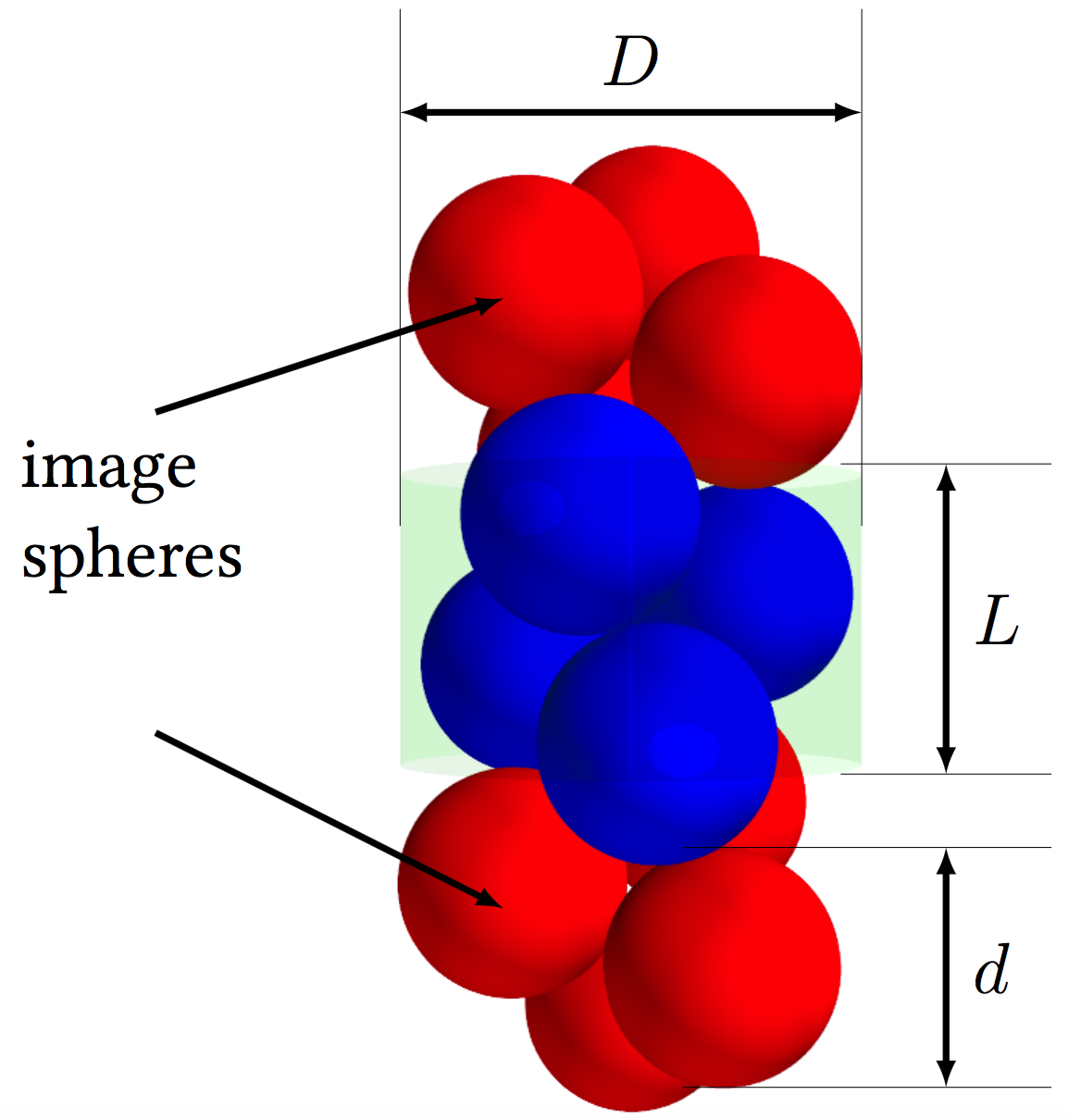
The soft sphere model in cylindrical confinement
The unit cell (blue spheres) of length \( L \) and diameter ratio \( D / d\) together with its image spheres (red), which allow us to simulate an infinite column.
Previous computer models have been simulating columnar packings of hard spheres, spheres that cannot overlap [Mughal12].
The only way to alter these structures is by varying the diameter ratio \( D/d \) between the tube diameter \(D\) and the sphere diameter \( d \).
All structures without inner spheres \( D/d < 2.7 \) have already been investigated intensively [] and provide a perfect starting point for our investigation of columnar sphere packings.
However, this crude model does not capture detailed properties like the deformation of the spheres.
Here we adopt the more accurate soft sphere model, where the contacting sphere have a repulsive potential, which allows the spheres to overlap.
But the inner energy \( U \) of the system increases quadratically in the overlap \( \delta_{ij} \).
In order to simulate an infinite column, we apply twisted periodic boundaries by using image spheres above and below the unit cell.
These image spheres are twisted by an angle \( \pm \alpha \).
To generate a packing of columnar soft spheres, we minimise the enthalpy \( H = U - pV \) for a given \( D / d \) and pressure \( p \):
$$H(\{r_i\}, L) = \frac{1}{2} k \sum_i^N \delta_{ij}^2 - p V.$$
This leaves the positions of the spheres \(r_i\), the twist angle \( \alpha \), and the tube length \( L \) (thus the volume \( V \)) as a minimisation variable.
Thus, packings are generated at constant pressure, but variable volume.
Simulation and observation of the \((3, \textbf{2}, 1)\) line slip
One particular type of structure with special relevance is the so called line-slip arrangement.
But before explaining the crucial significance of those structure, it is important to understand what those structures are and how they differ from uniform structures.
To classify these structures, we borough the so-called phyllotactic notation from botany.
In this notation a structure is described by three numbers \( (l, m, n) \), where each number represents a helix in a certain direction.
It requires a bit of practice to identify structures from this notation.
Thus, I will provide images in the following for all the major structures.
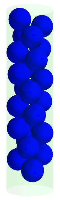
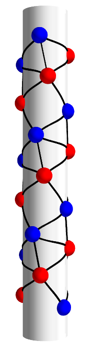
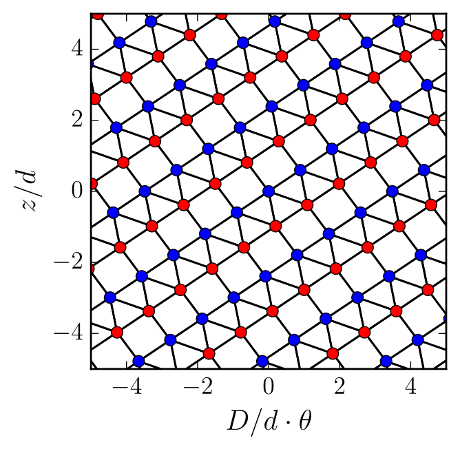
As an example, the \( (3, \textbf{2}, 1) \) line-slip structure is illustrated in the images below, first as the packing itself, then its contact network, and on the far right the rolled-out contact network.
From the contact network we can identify the special character of such structures:
While in uniform structures every sphere has always six contacts, in a line slip some spheres only have five contacts.
These gaps or loss of contacts appear always along a line (see rolled-out contact network) because the spheres with five contacts are slipped against each other.
\( (3, \textbf{2}, 1) \) line-slip packing of bubbles in a tube.
Contact network of the \( (3, \textbf{2}, 1) \) line-slip structure.
Corresponding rolled-out pattern of the contact network.
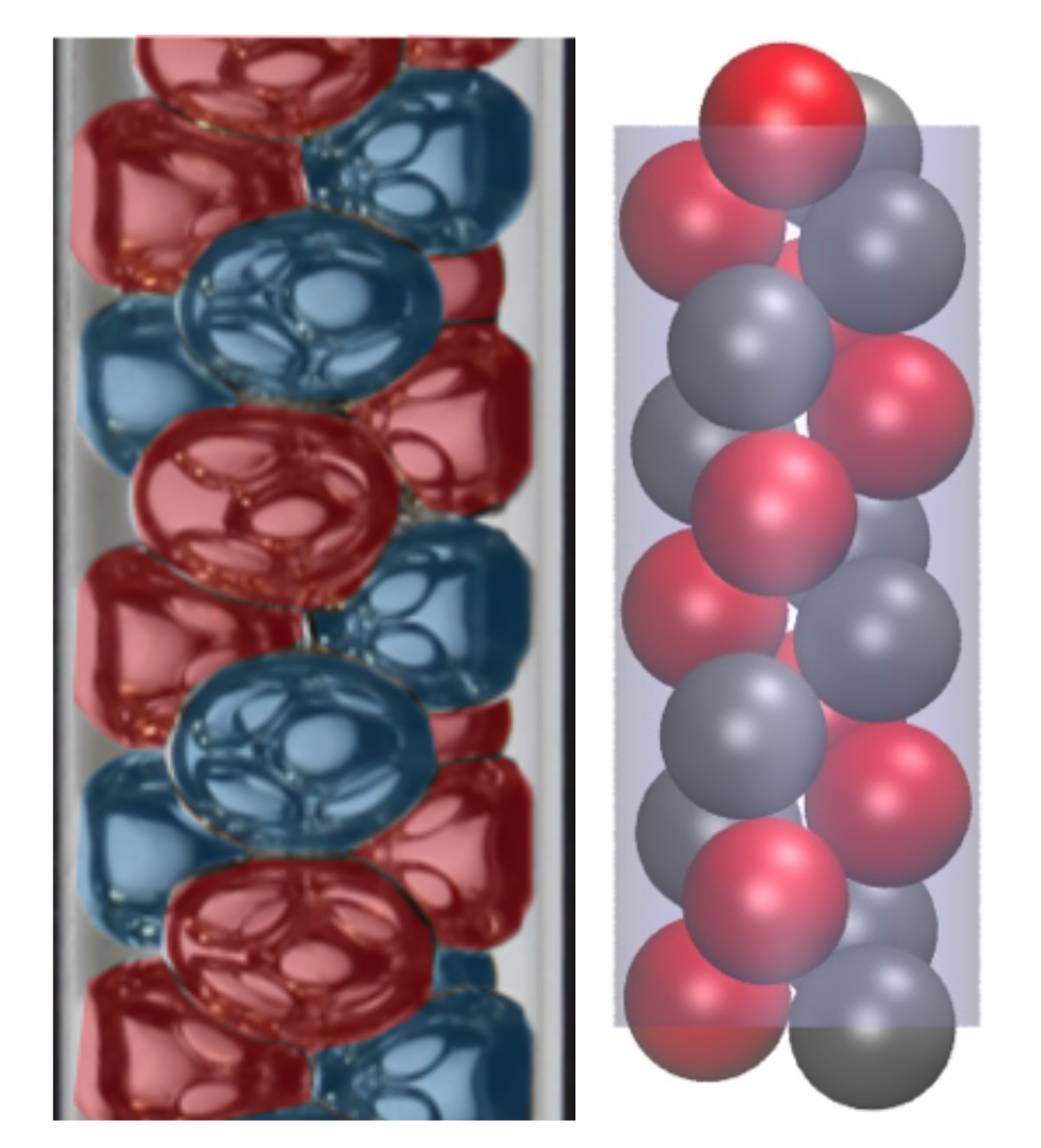
Newly discovered \( (3, \textbf{2}, 1) \) line slip of bubbles in a tube (left) in comparison with the simulated packing (right).
The loss of contact makes line-slip arrangements an interesting structure for many applications.
While uniform structure under pressure only compress by an increase of overlap, line slips can adjust the gap.
This makes line-slip structure compressible (up to 5%).
Experiments have shown that the existence of such structures are not only a fantasy of our computer simulations.
As a matter of fact, we were the first group to discover such a structure experimentally in a wet columnar foam [1].
Independent of us, a group in Harvard came upon a structure with a so-called line-slip defect in a colloidal crystal on a cylinder surface [Tanjeem18].
Further examples for such structures are currently under investigation.
After our simulation predicted the existence of such structures, we conducted experiments with wet foam columns inside a tube.
For the experimental set-up, monodisperse bubbles are produced by blowing air through a needle into a commercial surfactant Fairy Liquid.
The surfactant solution contained 50% of glycerol in mass to increase the viscosity, smooth the transition between structures and helps us to observe more easily unstable bubble arrangements.
Tuning the gas flow rate allowed us to produce monodisperse bubbles of controlled size.
The bubbles were then released into a tube from the bottom, where they self-assembled into a dry ordered foam.
The resulting foam column is put under forced drainage by feeding it with surfactant solution from the top.
This turned the the dry foam structure into a wet foam, where the spheres are approximately spherical as in our simulations.
In the figure on the side is an example of the observation of the \( (3, \textbf{2}, 1) \) line-slip structure in accord with expectations based on the soft sphere model.
Note that the bubbles are distorted into smooth ellipsoids by the flow.
This makes a direct comparison with our simulation difficult.
However, the extent of the loss of contact in the observed line-slip structure is roughly equal to the structure in the very center of the \( (3, \textbf{2}, 1) \) line-slip region in the phase diagram below.
The phase diagram of all ordered packings
Now that we know about the existence and the importance of such line slips, we would like to explore under which conditions they appear.
A look back at our model tells us, that the simulated structures only depend on the diameter ratio \( D / d \) and the pressure \( p \).
Thus, we mapped out a phase diagram for those two parameters by searching for the structure with the global enthalpy minimum at a given diameter ratio and pressure.
The video below shows the phase diagram of all columnar structures in the range of \( 1.5 \le D/d \le 2.7 \), together with the rolled-out contact network and the actual packing.
The upper limit of \( D/ d\) marks the point at which the character of the optimal structures changes radically; beyond this point the structures contain inner spheres which are not in contact with the cylindrical wall [18].
The pressure range is limited to \( p \le 0.02 \), beyond which line-slip structures are absent.
For pressures \( p = 0 \) our simulations resemble the hard sphere limit since the spheres do not overlap.
At this pressure we observe the same structure sequence with varying \( D / d\) as previous hard sphere simulations.
However, due to the restricted resolution the \( (\textbf{2}, 1, 1) \) and \( (\textbf{3}, 2, 1) \) are not visible in the phase diagram of the video below.
At large pressures the model may be regarded as unrealistic.
For a system of bubbles, which was the initial context for this work, one encounters the “dry limit”, as p increases, at which point all liquid in a foam has been removed.
The simulations were run with \( N = 3,4,5 \) spheres in the unit cell and for a given value of pressure and diameter ratio the structure with the lowest enthalpy was selected for the phase diagram.
Above the diameter ratio of 2.0, we find twenty-four distinct structures.
There are ten uniform packings and the remaining fourteen structures are their corresponding line slips.
Below \( D/d = 2.0 \) we observe the bamboo structure, the zigzag packing (i.e. the (2, 1, 1) uniform arrangement), and the twisted zigzag structure (i.e. the \( (2, \textbf{1}, 1) \) line slip).
The transitions between different structures can be classified as follows.
In continuous phase transitions (marked with dashed lines in Fig. 2) a structure transforms smoothly into another by gaining or losing a contact.
This can be observed in the video below, which shows an overview over all structures at a low pressure together with the corresponding rolled-out contact network and the structure’s position in the phase diagram.
This type of transition is found between a uniform structure and a line slip.
The zigzag to (2, 1, 1) transition is also continuous.
Discontinuous transitions (solid lines in phase diagram) are transitions where one structure changes abruptly into another (see also video).
The contact network of the packing (left), the phase diagram of all 27 columnar structures without inner spheres (center) and an image of the packing itself (right).
The moving black dot indicates the position in the phase diagram for the given packing and corresponding contact network.
In the phase diagram continuous phase transitions are marked with dashed lines, whereas discontinuous transitions appear at solid lines.
Stability diagrams of a selected transition
Whereas the computation of a phase diagram entailed a search for the global minimum of the enthalpy, involving an algorithm that allowed radical changes of structure to be explored, here we now pursue a more limited objective.
Given a stable structure, possibly metastable, how does it change when the pressure \( p \) and diameter ratio \( D/d \) are continuously varied, if it is to remain in the local minimum of enthalpy?
We do this by computing trajectories in the \( (p,D/d) \) plane, and recording boundaries where the structure changes to one of a different character.
With a sufficient number of trajectories, a stability diagram is built up, i.e. a map of the location of structural transitions.
In the following example we consider transitions between the (3,2,1) and (4,2,2) uniform structures and the associated \( (3, \textbf{2}, 1) \) line-slip.
We show that at a low pressures it is possible to start with any one of these structures and continuously transform one structure into another:
that is, a change in \( D/d \) can transform a uniform structure into a line-slip arrangement by the loss or formation of a contact.
However, at higher pressures these transitions are no longer reversible and show evidence of hysteresis, such discontinuous transformations are accompanied by a discontinuity in enthalpy.
From such results we eventually obtain a stability diagram operational for any trajectory taken in terms of \( D/d \) and \( p \).
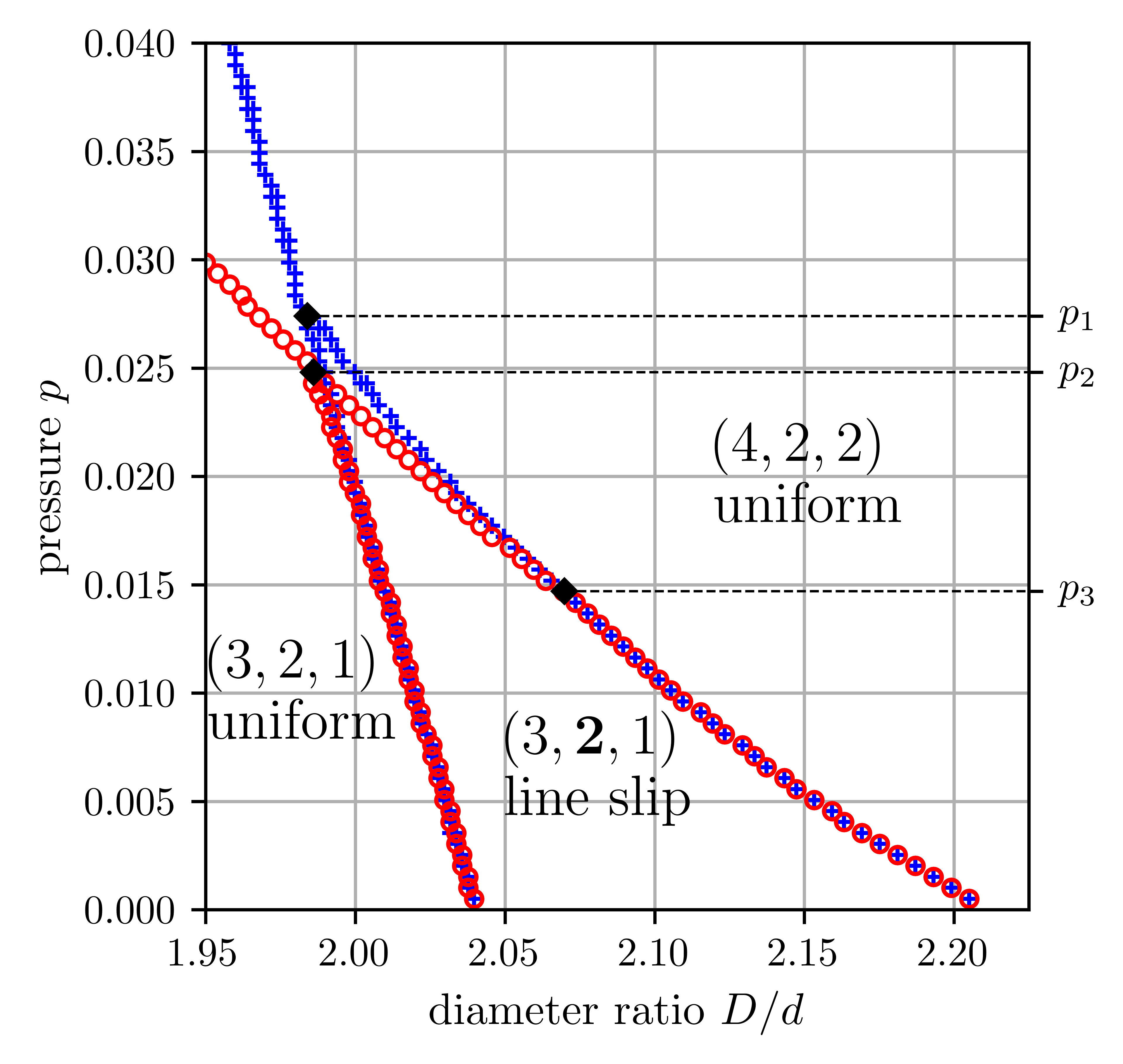
Stability diagram
The stability diagram for the (3, 2, 1) \( (3, \textbf{2}, 1) \) line-slip, and (4, 2, 2) structures.
The red circles indicate the boundaries for the stability regions, when increasing \( D/d \) from starting in a (3, 2, 1) uniform structure.
The blue crosses are the boundaries for the reversed trajectories, starting in the (4, 2, 2) and decreasing the diameter ratio.
From this diagram we can already see that the boundaries start to diverge for pressures above \( p_3 \), which indicates hysteresis.
The schematic diagram to the right will help us to interpret these results in more detail.
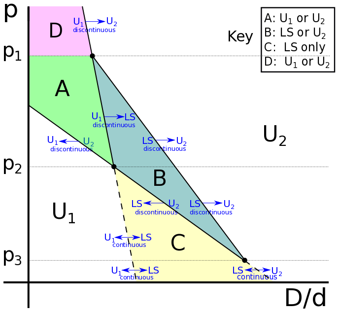
Schematic diagram
This schematic diagram is a schematic guide to the interpretation of the stability diagram, which is correct in representing the topological features of the stability diagram but does not preserve the geometrical features.
It show the continuous (dashed line) or discontinuous (solid line) boundaries, where the arrows indicate the directions for which such boundaries entail a transition.
Here the two uniform arrangements are labeled \( U_1 \) and \( U_2 \) and the intermediate line-slip arrangement is labeled LS.
With each new pressure regimes given by \( p_1 \) to \( p_3 \), a continuous boundary splits up into two discontinuous, which indicates hysteresis for all pressure regimes except the lowest one \( p < p_3 \).
To illustrate the useful application of the schematic diagram above I will describe the case \(p_3 \le p \le p_2 \) in detail here.
The other cases can be interpreted similarly by comparing the stability diagram with the schematic diagram.
The accompanied video below will illustrate the change in structure for the example case described here.
Starting from the (3, 2, 1) uniform packing at p = 0.020 increasing \( D/d \) leads to a boundary (shown by the blue crosses) which marks the continuous transition to the (3, 2, 1) line slip.
In the schematic diagram this is marked by the dashed line indicating the continuous transition \( U_1 \leftrightarrow LS \).
Increasing \( D/d \) further a second boundary (blue crosses) is encountered, making a discontinuous transition to the (4, 2, 2) uniform structure.
This boundary is shown in the schematic diagram by the solid line and is labeled \( LS \rightarrow U_2 \).
The arrow indicates that this is only encountered upon increasing \( D/d \), transforming the line-slip \(LS \) into the uniform structure \( U_2 \) by a discontinuous transition.
Upon decreasing \( D/d \) the (4, 2, 2) uniform structure undergoes a discontinuous transition at the boundary indicated by red dots in the stability diagram into the (3, 2, 1) line-slip.
This boundary is marked by the solid line in the schematic diagram accompanied by the label \( LS \leftarrow U_2 \).
A further decrease of \( D/d \) results in a continuous transition into the uniform (3, 2, 1) structure, at the boundary marked by red dots in the stability diagram and dashed line in the schematic diagram.
We have thus returned to the starting point of this particular excursion through the stability diagram.
The contact network (left), the stability map (center), showing the transition lines between \( (3, 2, 1) \), \( (3, \textbf{2}, 1) \) and \( (4, 2, 2) \), and an image of the packing itself (right).
The moving black dot indicates again the position in the stability map for the given packing and corresponding contact network.
Lorem ipsum dolor sit amet, consectetuer adipiscing
elit. Aenean commodo ligula eget dolor. Aenean massa.
Cum sociis natoque penatibus et magnis dis parturient
montes, nascetur ridiculus mus. Donec quam felis,
ultricies nec, pellentesque eu, pretium quis, sem.
Plat
A very popular open-source 2D foam simulation created by F. Bolton in our group is Plat.
Its source code can be found in this git repository.
Lorem ipsum dolor sit amet, consectetuer adipiscing
elit. Aenean commodo ligula eget dolor. Aenean massa.
Cum sociis natoque penatibus et magnis dis parturient
montes.
The soft disk model
Lorem ipsum dolor sit amet, consectetuer adipiscing
elit. Aenean commodo ligula eget dolor. Aenean massa.
Cum sociis natoque penatibus et magnis dis parturient
montes, nascetur ridiculus mus. Donec quam felis,
ultricies nec, pellentesque eu, pretium quis, sem.
The Morse-Witten model
Lorem ipsum dolor sit amet, consectetuer adipiscing
elit. Aenean commodo ligula eget dolor. Aenean massa.
Cum sociis natoque penatibus et magnis dis parturient
montes, nascetur ridiculus mus. Donec quam felis,
ultricies nec, pellentesque eu, pretium quis, sem.
Further reading:
[1] Winkelmann J., Dunne F.F., Langlois V.J., Möbius M.E., Weaire D., Hutzler S. (2017) 2d foams above the jamming transition: Deformation matters, Colloids and Surfaces A: Physicochemical and Engineering Aspects 534 52–57
Multi-Particle Collision Dynamics (MPCD)
This is a hydrodynamic simulation method, used for simulations ranging from active matter to polymers.
In my master thesis at TU Dortmund I used it to simulate the hydrodynamic interaction between two polymers in a cubed channel and compared results to experiments.
Since this was quite a while ago and I am too lazy to read it again, I will probably not write anything about it here.
Feel free to read my master thesis, though!