1 Introduction
1.1 A brief history
The last century saw an expansion in our view of the world from a static, Galaxy-sized Universe, whose constituents were stars and “nebulae” of unknown but possibly stellar origin, to the view that the observable Universe is in a state of expansion from an initial singularity over ten billion years ago, and contains approximately 100 billion galaxies. This paradigm shift was summarised in a famous debate between Shapley and Curtis in 1920; summaries of the views of each protagonist can be found in [43] and [195].
The historical background to this change in world view has been extensively discussed and whole books have been devoted to the subject of distance measurement in astronomy [176*]. At the heart of the change was the conclusive proof that what we now know as external galaxies lay at huge distances, much greater than those between objects in our own Galaxy. The earliest such distance determinations included those of the galaxies NGC 6822 [93], M33 [94] and M31 [96], by Edwin Hubble.
As well as determining distances, Hubble also considered redshifts of spectral lines in galaxy spectra
which had previously been measured by Slipher in a series of papers [197, 198]. If a spectral
line of emitted wavelength  is observed at a wavelength
  , the redshift
  is defined as

 which for nearby objects behaves in a way predicted by a simple Doppler
formula,1
which for nearby objects behaves in a way predicted by a simple Doppler
formula,1
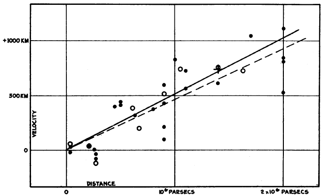
 . Hubble showed that a relation existed between distance and redshift (see Figure 1*); more distant
galaxies recede faster, an observation which can naturally be explained if the Universe as a whole is
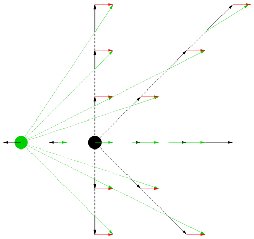
expanding. The relation between the recession velocity and distance is linear in nearby objects, as it must
be if the same dependence is to be observed from any other galaxy as it is from our own Galaxy (see
Figure 2*). The proportionality constant is the Hubble constant
. Hubble showed that a relation existed between distance and redshift (see Figure 1*); more distant
galaxies recede faster, an observation which can naturally be explained if the Universe as a whole is
expanding. The relation between the recession velocity and distance is linear in nearby objects, as it must
be if the same dependence is to be observed from any other galaxy as it is from our own Galaxy (see
Figure 2*). The proportionality constant is the Hubble constant  , where the subscript indicates a value
as measured now. Unless the Universe’s expansion does not accelerate or decelerate, the slope of the
velocity–distance relation is different for observers at different epochs of the Universe. As well as the
velocity corresponding to the universal expansion, a galaxy also has a “peculiar velocity”, typically of
a few hundred kms–1, due to groups or clusters of galaxies in its vicinity. Peculiar velocities
are a nuisance if determining the Hubble constant from relatively nearby objects for which
they are comparable to the recession velocity. Once the distance is
, where the subscript indicates a value
as measured now. Unless the Universe’s expansion does not accelerate or decelerate, the slope of the
velocity–distance relation is different for observers at different epochs of the Universe. As well as the
velocity corresponding to the universal expansion, a galaxy also has a “peculiar velocity”, typically of
a few hundred kms–1, due to groups or clusters of galaxies in its vicinity. Peculiar velocities
are a nuisance if determining the Hubble constant from relatively nearby objects for which
they are comparable to the recession velocity. Once the distance is  50 Mpc, the recession
velocity is large enough for the error in
50 Mpc, the recession
velocity is large enough for the error in  due to the peculiar velocity to be less than about
10%.
due to the peculiar velocity to be less than about
10%.
Recession velocities are very easy to measure; all we need is an object with an emission line and a
spectrograph. Distances are very difficult. This is because in order to measure a distance, we need a
standard candle (an object whose luminosity is known) or a standard ruler (an object whose length is
known), and we then use apparent brightness or angular size to work out the distance. Good standard
candles and standard rulers are in short supply because most such objects require that we understand
their astrophysics well enough to work out what their luminosity or size actually is. Neither
stars nor galaxies by themselves remotely approach the uniformity needed; even when selected
by other, easily measurable properties such as colour, they range over orders of magnitude in
luminosity and size for reasons that are astrophysically interesting but frustrating for distance
measurement. The ideal  object, in fact, is one which involves as little astrophysics as
possible.
object, in fact, is one which involves as little astrophysics as
possible.
Hubble originally used a class of stars known as Cepheid variables for his distance determinations. These
are giant blue stars, the best known of which is  UMa, or Polaris. In most normal stars, a self-regulating
mechanism exists in which any tendency for the star to expand or contract is quickly damped out. In a small
range of temperature on the Hertzsprung–Russell (H-R) diagram, around 7000 – 8000 K, particularly at high
luminosity,2
this does not happen and pulsations occur. These pulsations, the defining property of Cepheids, have a
characteristic form, a steep rise followed by a gradual fall. They also have a period which is directly
proportional to luminosity, because brighter stars are larger, and therefore take longer to pulsate. The
period-luminosity relationship was discovered by Leavitt [123] by studying a sample of Cepheid
variables in the Large Magellanic Cloud (LMC). Because these stars were known to be all at
the same distance, their correlation of apparent magnitude with period therefore implied the
P-L relationship.
UMa, or Polaris. In most normal stars, a self-regulating
mechanism exists in which any tendency for the star to expand or contract is quickly damped out. In a small
range of temperature on the Hertzsprung–Russell (H-R) diagram, around 7000 – 8000 K, particularly at high
luminosity,2
this does not happen and pulsations occur. These pulsations, the defining property of Cepheids, have a
characteristic form, a steep rise followed by a gradual fall. They also have a period which is directly
proportional to luminosity, because brighter stars are larger, and therefore take longer to pulsate. The
period-luminosity relationship was discovered by Leavitt [123] by studying a sample of Cepheid
variables in the Large Magellanic Cloud (LMC). Because these stars were known to be all at
the same distance, their correlation of apparent magnitude with period therefore implied the
P-L relationship.
The Hubble constant was originally measured as  [95] and its subsequent
history was a more-or-less uniform revision downwards. In the early days this was caused by
bias3
in the original samples [12], confusion between bright stars and H ii regions
in the original samples [97, 185] and differences between type I and II
Cepheids4
[7]. In the second half of the last century, the subject was dominated by a lengthy dispute between investigators
favouring values around
[95] and its subsequent
history was a more-or-less uniform revision downwards. In the early days this was caused by
bias3
in the original samples [12], confusion between bright stars and H ii regions
in the original samples [97, 185] and differences between type I and II
Cepheids4
[7]. In the second half of the last century, the subject was dominated by a lengthy dispute between investigators
favouring values around  and those preferring higher values of
  .
Most astronomers would now bet large amounts of money on the true value lying between these extremes,
and this review is an attempt to explain why and also to try and evaluate the evidence for the best-guess
current value. It is not an attempt to review the global history of
.
Most astronomers would now bet large amounts of money on the true value lying between these extremes,
and this review is an attempt to explain why and also to try and evaluate the evidence for the best-guess
current value. It is not an attempt to review the global history of  determinations, as this has been
done many times, often by the original protagonists or their close collaborators. For an overall review of
this process see, for example, [223] and [210]. Compilations of data and analysis of them are
given by Huchra (
determinations, as this has been
done many times, often by the original protagonists or their close collaborators. For an overall review of
this process see, for example, [223] and [210]. Compilations of data and analysis of them are
given by Huchra ( http://cfa-www.harvard.edu/~huchra/hubble), and Gott ([77], updated
by [35]).5
Further reviews of the subject, with various different emphases and approaches, are given by [212, 68*].
http://cfa-www.harvard.edu/~huchra/hubble), and Gott ([77], updated
by [35]).5
Further reviews of the subject, with various different emphases and approaches, are given by [212, 68*].
In summary, the ideal object for measuring the Hubble constant:
- Has a property which allows it to be treated as either as a standard candle or as a standard ruler
- Can be used independently of other calibrations (i.e., in a one-step process)
- Lies at a large enough distance (a few tens of Mpc or greater) that peculiar velocities are small compared to the recession velocity at that distance
- Involves as little astrophysics as possible, so that the distance determination does not depend on internal properties of the object
- Provides the Hubble constant independently of other cosmological parameters.
Many different methods are discussed in this review. We begin with one-step methods, and in particular
with the use of megamasers in external galaxies – arguably the only method which satisfies all the above
criteria. Two other one-step methods, gravitational lensing and Sunyaev–Zel’dovich measurements, which
have significant contaminating astrophysical effects are also discussed. The review then discusses two other
programmes: first, the Cepheid-based distance ladders, where the astrophysics is probably now well
understood after decades of effort, but which are not one-step processes; and second, information from the
CMB, an era where astrophysics is in the linear regime and therefore simpler, but where  is not
determined independently of other cosmological parameters in a single experiment, without further
assumptions.
is not
determined independently of other cosmological parameters in a single experiment, without further
assumptions.
1.2 A little cosmology
The expanding Universe is a consequence, although not the only possible consequence, of general relativity coupled with the assumption that space is homogeneous (that is, it has the same average density of matter at all points at a given time) and isotropic (the same in all directions). In 1922, Friedman [72] showed that given that assumption, we can use the Einstein field equations of general relativity to write down the dynamics of the Universe using the following two equations, now known as the Friedman equations:
Here
 is the scale factor of the Universe. It is fundamentally related to redshift, because the
quantity
is the scale factor of the Universe. It is fundamentally related to redshift, because the
quantity  is the ratio of the scale of the Universe now to the scale of the Universe at the time of
emission of the light (
is the ratio of the scale of the Universe now to the scale of the Universe at the time of
emission of the light ( ).
).  is the cosmological constant, which appears in the field
equation of general relativity as an extra term. It corresponds to a universal repulsion and
was originally introduced by Einstein to coerce the Universe into being static. On Hubble’s
discovery of the expansion of the Universe, he removed it, only for it to reappear seventy years
later as a result of new data [157*, 169*] (see also [34*, 235*] for a review).
is the cosmological constant, which appears in the field
equation of general relativity as an extra term. It corresponds to a universal repulsion and
was originally introduced by Einstein to coerce the Universe into being static. On Hubble’s
discovery of the expansion of the Universe, he removed it, only for it to reappear seventy years
later as a result of new data [157*, 169*] (see also [34*, 235*] for a review).  is a curvature
term, and is
is a curvature
term, and is  ,
,  , or
, or  , according to whether the global geometry of the Universe is
negatively curved, spatially flat, or positively curved.
, according to whether the global geometry of the Universe is
negatively curved, spatially flat, or positively curved.  is the density of the contents of the
Universe,
is the density of the contents of the
Universe,  is the pressure and dots represent time derivatives. For any particular component of
the Universe, we need to specify an equation for the relation of pressure to density to solve
these equations; for most components of interest such an equation is of the form
is the pressure and dots represent time derivatives. For any particular component of
the Universe, we need to specify an equation for the relation of pressure to density to solve
these equations; for most components of interest such an equation is of the form  .
Component densities vary with scale factor
.
Component densities vary with scale factor  as the Universe expands, and hence vary with
time.
as the Universe expands, and hence vary with
time.
At any given time, we can define a Hubble parameter
which is obviously related to the Hubble constant, because it is the ratio of an increase in scale factor to the scale factor itself. In fact, the Hubble constant
 is just the value of
  at the current
time.6
at the current
time.6
If  , we can derive the kinematics of the Universe quite simply from the first Friedman equation.
For a spatially flat Universe
, we can derive the kinematics of the Universe quite simply from the first Friedman equation.
For a spatially flat Universe  , and we therefore have

 is known as the critical density. For Universes whose densities are less than this
critical density,
is known as the critical density. For Universes whose densities are less than this
critical density,  and space is negatively curved. For such Universes it is easy to see
from the first Friedman equation that we require
and space is negatively curved. For such Universes it is easy to see
from the first Friedman equation that we require  , and therefore the Universe must
carry on expanding for ever. For positively curved Universes (
, and therefore the Universe must
carry on expanding for ever. For positively curved Universes ( ), the right hand side is
negative, and we reach a point at which
), the right hand side is
negative, and we reach a point at which  . At this point the expansion will stop and
thereafter go into reverse, leading eventually to a Big Crunch as
. At this point the expansion will stop and
thereafter go into reverse, leading eventually to a Big Crunch as  becomes larger and more
negative.
becomes larger and more
negative.
For the global history of the Universe in models with a cosmological constant, however, we need to
consider the  term as providing an effective acceleration. If the cosmological constant is
positive, the Universe is almost bound to expand forever, unless the matter density is very much
greater than the energy density in cosmological constant and can collapse the Universe before the
acceleration takes over. (A negative cosmological constant will always cause recollapse, but is
not part of any currently likely world model). Carroll [34] provides further discussion of this
point.
term as providing an effective acceleration. If the cosmological constant is
positive, the Universe is almost bound to expand forever, unless the matter density is very much
greater than the energy density in cosmological constant and can collapse the Universe before the
acceleration takes over. (A negative cosmological constant will always cause recollapse, but is
not part of any currently likely world model). Carroll [34] provides further discussion of this
point.
We can also introduce some dimensionless symbols for energy densities in the cosmological constant at
the current time,  , and in “curvature energy”,
  . By rearranging the first
Friedman equation we obtain
. By rearranging the first
Friedman equation we obtain

The density in a particular component of the Universe  , as a fraction of critical density, can be
written as
, as a fraction of critical density, can be
written as

 represents the dilution of the component as the Universe expands. It is related to
the
represents the dilution of the component as the Universe expands. It is related to
the  parameter defined earlier by the equation
  . For ordinary matter
  , and for
radiation
, and for
radiation  , because in addition to geometrical dilution as the universe expands, the energy of
radiation decreases as the wavelength increases. The cosmological constant energy density remains the same
no matter how the size of the Universe increases, hence for a cosmological constant we have
, because in addition to geometrical dilution as the universe expands, the energy of
radiation decreases as the wavelength increases. The cosmological constant energy density remains the same
no matter how the size of the Universe increases, hence for a cosmological constant we have  and
and
 .
.  is not the only possibility for producing acceleration, however. Any general class of
“quintessence” models for which
is not the only possibility for producing acceleration, however. Any general class of
“quintessence” models for which  will do; the case
  is probably the most
extreme and eventually results in the accelerating expansion becoming so dominant that all
gravitational interactions become impossible due to the shrinking boundary of the observable
Universe, finally resulting in all matter being torn apart in a “Big Rip” [32]. In current models
is probably the most
extreme and eventually results in the accelerating expansion becoming so dominant that all
gravitational interactions become impossible due to the shrinking boundary of the observable
Universe, finally resulting in all matter being torn apart in a “Big Rip” [32]. In current models  will become increasingly dominant in the dynamics of the Universe as it expands. Note that
by definition, because
will become increasingly dominant in the dynamics of the Universe as it expands. Note that
by definition, because 
 implies a flat Universe in which the total energy density in matter together
with the cosmological constant is equal to the critical density. Universes for which
implies a flat Universe in which the total energy density in matter together
with the cosmological constant is equal to the critical density. Universes for which  is almost zero
tend to evolve away from this point, so the observed near-flatness is a puzzle known as the
“flatness problem”; the hypothesis of a period of rapid expansion known as inflation in the early
history of the Universe predicts this near-flatness naturally. As well as a solution to the flatness
problem, inflation is an attractive idea because it provides a natural explanation for the large-scale
uniformity of the Universe in regions which would otherwise not be in causal contact with each
other.
is almost zero
tend to evolve away from this point, so the observed near-flatness is a puzzle known as the
“flatness problem”; the hypothesis of a period of rapid expansion known as inflation in the early
history of the Universe predicts this near-flatness naturally. As well as a solution to the flatness
problem, inflation is an attractive idea because it provides a natural explanation for the large-scale
uniformity of the Universe in regions which would otherwise not be in causal contact with each
other.
We finally obtain an equation for the variation of the Hubble parameter with time in terms of the Hubble constant (see, e.g., [155]),
where
 represents the energy density in radiation and
  the energy density in matter.
To obtain cosmological distances, we need to perform integrals of the form
where the right-hand side can be expressed as a “Hubble distance”
 , multiplied by an integral
over dimensionless quantities such as the
, multiplied by an integral
over dimensionless quantities such as the  terms. We can define a number of distances in cosmology,
including the “comoving” distance
terms. We can define a number of distances in cosmology,
including the “comoving” distance  defined above. The most important for present purposes
are the angular diameter distance
defined above. The most important for present purposes
are the angular diameter distance  , which relates the apparent angular
size of an object to its proper size, and the luminosity distance
, which relates the apparent angular
size of an object to its proper size, and the luminosity distance  , which
relates the observed flux of an object to its intrinsic luminosity. For currently popular models,
the angular diameter distance increases to a maximum as
, which
relates the observed flux of an object to its intrinsic luminosity. For currently popular models,
the angular diameter distance increases to a maximum as  increases to a value of order 1,
and decreases thereafter. Formulae for, and fuller explanations of, both distances are given
by [87].
increases to a value of order 1,
and decreases thereafter. Formulae for, and fuller explanations of, both distances are given
by [87].
 |
 |
 |