List of Figures
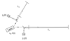 |
Figure 1:
Light from a laser is split into two beams, each injected into an arm formed by pairs of free-falling mirrors. Since the length of the two arms,  and and  , are different, now the light
beams from the two arms are not recombined at one photo detector. Instead each is separately made
to interfere with the light that is injected into the arms. Two distinct photo detectors are now used,
and phase (or frequency) fluctuations are then monitored and recorded there. , are different, now the light
beams from the two arms are not recombined at one photo detector. Instead each is separately made
to interfere with the light that is injected into the arms. Two distinct photo detectors are now used,
and phase (or frequency) fluctuations are then monitored and recorded there. |
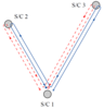 |
Figure 2:
Schematic diagram for  , showing that it is a synthesized zero-area Sagnac
interferometer. The optical path begins at an “x” and the measurement is made at an “o”. , showing that it is a synthesized zero-area Sagnac
interferometer. The optical path begins at an “x” and the measurement is made at an “o”. |
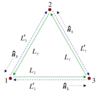 |
Figure 3:
Schematic LISA configuration. The spacecraft are labeled 1, 2, and 3. The optical paths are denoted by  , ,  where the index where the index  corresponds to the opposite spacecraft. The unit
vectors corresponds to the opposite spacecraft. The unit
vectors  point between pairs of spacecraft, with the orientation indicated. point between pairs of spacecraft, with the orientation indicated. |
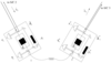 |
Figure 4:
Schematic diagram of proof-masses-plus-optical-benches for a LISA spacecraft. The left-hand bench reads out the phase signals  and and  . The right-hand bench analogously reads
out . The right-hand bench analogously reads
out  and and  . The random displacements of the two proof masses and two optical benches are
indicated (lower case . The random displacements of the two proof masses and two optical benches are
indicated (lower case  for the proof masses, upper case for the proof masses, upper case  for the optical benches). for the optical benches). |
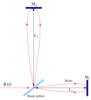 |
Figure 5:
Schematic diagram of the unequal-arm Michelson interferometer. The beam shown corresponds to the term  in in  which is first sent around arm 1 followed
by arm 2. The second beam (not shown) is first sent around arm 2 and then through arm 1. The
difference in these two beams constitutes which is first sent around arm 1 followed
by arm 2. The second beam (not shown) is first sent around arm 2 and then through arm 1. The
difference in these two beams constitutes  . . |
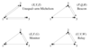 |
Figure 6:
Schematic diagrams of the unequal-arm Michelson, Monitor, Beacon, and Relay combinations. These TDI combinations rely only on four of the six one-way Doppler measurements, as illustrated here. |
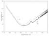 |
Figure 7:
The LISA Michelson sensitivity curve (SNR = 5) and the sensitivity curve for the optimal combination of the data, both as a function of Fourier frequency. The integration time is equal to one year, and LISA is assumed to have a nominal armlength  = 16.67 s. = 16.67 s. |
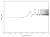 |
Figure 8:
The optimal SNR divided by the SNR of a single Michelson interferometer, as a function of the Fourier frequency  . The sensitivity gain in the low-frequency band is equal to . The sensitivity gain in the low-frequency band is equal to  , while
it can get larger than 2 at selected frequencies in the high-frequency region of the accessible band.
The integration time has been assumed to be one year, and the proof mass and optical path noise
spectra are the nominal ones. See the main body of the paper for a quantitative discussion of this
point. , while
it can get larger than 2 at selected frequencies in the high-frequency region of the accessible band.
The integration time has been assumed to be one year, and the proof mass and optical path noise
spectra are the nominal ones. See the main body of the paper for a quantitative discussion of this
point. |
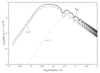 |
Figure 9:
The SNRs of the three combinations  and their sum as a function of the Fourier
frequency and their sum as a function of the Fourier
frequency  . The SNRs of . The SNRs of  and and  are equal over the entire frequency band. The SNR of are equal over the entire frequency band. The SNR of  is significantly smaller than the other two in the low part of the frequency band, while is comparable
to (and at times larger than) the SNR of the other two in the high-frequency region. See text for a
complete discussion.
is significantly smaller than the other two in the low part of the frequency band, while is comparable
to (and at times larger than) the SNR of the other two in the high-frequency region. See text for a
complete discussion. |
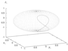 |
Figure 10:
Apparent position of the source in the sky as seen from LISA frame for  . The track of the source for a period of one year is shown on the unit sphere
in the LISA reference frame. . The track of the source for a period of one year is shown on the unit sphere
in the LISA reference frame. |
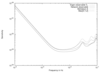 |
Figure 11:
Sensitivity curves for the observables: Michelson, ![max [X, Y,Z ]](article876x.gif) , ,  , and network for
the source direction ( , and network for
the source direction ( , ,  ). ). |
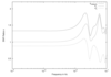 |
Figure 12:
Ratios of the sensitivities of the observables network,  with with ![max [X, Y,Z ]](article882x.gif) for the
source direction for the
source direction  , ,  . . |
Massimo Tinto and Sanjeev V. Dhurandhar, "Time-Delay Interferometry",
Living Rev. Relativity, 17 (2014), 6, doi:10.12942/lrr-2014-6, URL (accessed <date>): http://www.livingreviews.org/lrr-2014-6. This work is licensed under a Creative Commons License.
© The author(s), except where otherwise noted.
This work is licensed under a Creative Commons License.
© The author(s), except where otherwise noted.
Living Rev. Relativity, 17 (2014), 6, doi:10.12942/lrr-2014-6, URL (accessed <date>): http://www.livingreviews.org/lrr-2014-6.
This work is licensed under a Creative Commons License.
© The author(s), except where otherwise noted.