3 Detectors
3.1 Gravitational-wave interferometers
Kilometer-scale gravitational-wave interferometers have been in operation for over a decade. These types of detectors use laser interferometry to monitor the locations of test masses at the ends of the arms with exquisite precision. Gravitational waves change the relative length of the optical cavities in the interferometer (or equivalently, the proper travel time of photons) resulting in a strain

 is the path length difference between the two arms of the interferometer.
Fractional changes in the difference in path lengths along the two arms can be monitored to better than
1 part in  . It is not hard to understand how such precision can be achieved. For a simple Michelson
interferometer, a difference in path length of order the size of a fringe can easily be detected. For the
typically-used, infrared lasers of wavelength
. It is not hard to understand how such precision can be achieved. For a simple Michelson
interferometer, a difference in path length of order the size of a fringe can easily be detected. For the
typically-used, infrared lasers of wavelength  , and interferometer arms of length
  , the
minimum detectable strain is
, the
minimum detectable strain is
This is still far off the  mark. In principle, however, changes in the length of the
cavities corresponding to fractions of a single fringe can also be measured provided we have a
sensitive photodiode at the dark port of the interferometer, and enough photons to perform the
measurement. This way we can track changes in the amount of light incident on the photodiode as the
lengths of the arms change and we move over a fringe. The rate at which photons arrive at the
photodiode is a Poisson process and the fluctuations in the number of photons is
mark. In principle, however, changes in the length of the
cavities corresponding to fractions of a single fringe can also be measured provided we have a
sensitive photodiode at the dark port of the interferometer, and enough photons to perform the
measurement. This way we can track changes in the amount of light incident on the photodiode as the
lengths of the arms change and we move over a fringe. The rate at which photons arrive at the
photodiode is a Poisson process and the fluctuations in the number of photons is  , where
 is the number of photons. Therefore we can track changes in the path length difference of
order
is the number of photons. Therefore we can track changes in the path length difference of
order

 , and the amount of time available to perform the
measurement. For a gravitational wave of frequency
, and the amount of time available to perform the
measurement. For a gravitational wave of frequency  , we can collect photons for a time
  , so the
number of photons is
, so the
number of photons is

 is Planck’s constant and
  is the laser frequency. For a typical laser power
 , a gravitational-wave frequency
  , and
, and  the number of photons
is
the number of photons
is


The sensitivity can be further improved by increasing the effective length of the arms. In the LIGO instruments, for example, each of the two arms forms a resonant Fabry–Pérot cavity. For gravitational-wave frequencies smaller than the inverse of the light storage time, the light in the cavities makes many back and forth trips in the arms, while the wave is traversing the instrument. For gravitational waves of frequencies around 100 Hz and below, the light makes about a thousand back and forth trips while the gravitational wave is traversing the interferometer, which results in a three-orders-of-magnitude improvement in sensitivity,

The proper light travel time of photons in interferometers is controlled by the metric perturbation, which can be expressed as a sum over polarization modes
where
 labels the six possible polarization modes in metric theories of gravity. The metric perturbation
for each mode can be written in terms of a plane wave expansion,
Here
labels the six possible polarization modes in metric theories of gravity. The metric perturbation
for each mode can be written in terms of a plane wave expansion,
Here 
 is the frequency of the gravitational waves,
  is the wave vector,
  is
a unit vector that points in the direction of propagation of the gravitational waves,
is
a unit vector that points in the direction of propagation of the gravitational waves,  is
the
is
the  th polarization tensor, with
  spatial indices. The metric perturbation
due to mode
spatial indices. The metric perturbation
due to mode  from the direction
  can be written by integrating over all frequencies,
By integrating Eq. (50*) over all frequencies we have an expression for the metric perturbation from a
particular direction
can be written by integrating over all frequencies,
By integrating Eq. (50*) over all frequencies we have an expression for the metric perturbation from a
particular direction 
 , i.e., only a function of
  . The full metric perturbation due to a
gravitational wave from a direction
. The full metric perturbation due to a
gravitational wave from a direction  can be written as a sum over all polarization modes

The response of an interferometer to gravitational waves is generally referred to as the antenna pattern
response, and depends on the geometry of the detector and the direction and polarization of the
gravitational wave. To derive the antenna pattern response of an interferometer for all six polarization
modes we follow the discussion in [329*] closely. For a gravitational wave propagating in the  direction,
the polarization tensors are as follows
direction,
the polarization tensors are as follows
 ,
,  ,
,  ,
,  ,
,  , and
, and  correspond to the plus, cross, vector-x, vector-y,
breathing, and longitudinal modes.
correspond to the plus, cross, vector-x, vector-y,
breathing, and longitudinal modes.
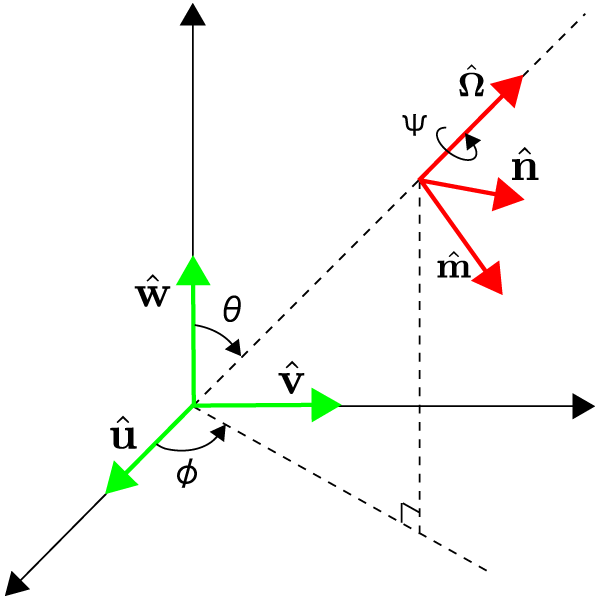
Suppose that the coordinate system for the detector is  ,
,  ,
,  , as
in Figure 1*. Relative to the detector, the gravitational-wave coordinate system is rotated by angles
, as
in Figure 1*. Relative to the detector, the gravitational-wave coordinate system is rotated by angles  ,
,
 ,
,  , and
, and  . We
still have the freedom to perform a rotation about the gravitational-wave propagation direction, which
introduces the polarization angle
. We
still have the freedom to perform a rotation about the gravitational-wave propagation direction, which
introduces the polarization angle  ,
,
The coordinate systems  and
and  are also shown in Figure 1*. To generalize the
polarization tensors in Eq. (53*) to a wave coming from a direction
are also shown in Figure 1*. To generalize the
polarization tensors in Eq. (53*) to a wave coming from a direction  , we use the unit vectors
  ,
,  ,
and
,
and  as follows

 and polarization angle
  takes the form
Explicitly, the antenna pattern functions are,
The dependence on the polarization angles
takes the form
Explicitly, the antenna pattern functions are,
The dependence on the polarization angles 
 reveals that the
  and
and  polarizations are spin-2
tensor modes, the
polarizations are spin-2
tensor modes, the  and
and  polarizations are spin-1 vector modes, and the
  and
and  polarizations are
spin-0 scalar modes. Note that for interferometers the antenna pattern responses of the scalar modes are
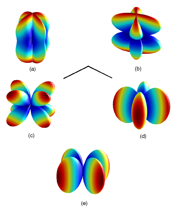
degenerate. Figure 2* shows the antenna patterns for the various polarizations given in Eq. (58*) with
polarizations are
spin-0 scalar modes. Note that for interferometers the antenna pattern responses of the scalar modes are
degenerate. Figure 2* shows the antenna patterns for the various polarizations given in Eq. (58*) with
 . The color indicates the strength of the response with red being the strongest and blue being the
weakest.
. The color indicates the strength of the response with red being the strongest and blue being the
weakest.
 .
Panels (a) and (b) show the plus (
.
Panels (a) and (b) show the plus ( ) and cross (
 ) modes, panels (c) and (d) the vector
x and vector y modes (
) modes, panels (c) and (d) the vector
x and vector y modes ( and
and  ), and panel (e) shows the scalar modes (up to a sign, it is
the same for both breathing and longitudinal). Color indicates the strength of the response with red
being the strongest and blue being the weakest. The black lines near the center give the orientation
of the interferometer arms.
), and panel (e) shows the scalar modes (up to a sign, it is
the same for both breathing and longitudinal). Color indicates the strength of the response with red
being the strongest and blue being the weakest. The black lines near the center give the orientation
of the interferometer arms.3.2 Pulsar timing arrays
Neutron stars can emit powerful beams of radio waves from their magnetic poles. If the rotational and magnetic axes are not aligned, the beams sweep through space like the beacon on a lighthouse. If the line of sight is aligned with the magnetic axis at any point during the neutron star’s rotation the star is observed as a source of periodic radio-wave bursts. Such a neutron star is referred to as a pulsar. Due to their large moment of inertia pulsars are very stable rotators, and their radio pulses arrive on Earth with extraordinary regularity. Pulsar timing experiments exploit this regularity: gravitational waves are expected to cause fluctuations in the time of arrival of radio pulses from pulsars.
The effect of a gravitational wave on the pulses propagating from a pulsar to Earth was first computed in the late 1970s by Sazhin and Detweiler [378, 145]. Gravitational waves induce a redshift in the pulse train
where
 is a unit vector that points in the direction of the pulsar,
  is the unit vector of gravitational
wave propagation, and
is the difference in the metric perturbation at the pulsar when the pulse was emitted and the metric
perturbation on Earth when the pulse was received. The inner product in Eq. (59*) is computed with the
Euclidean metric.
is the unit vector of gravitational
wave propagation, and
is the difference in the metric perturbation at the pulsar when the pulse was emitted and the metric
perturbation on Earth when the pulse was received. The inner product in Eq. (59*) is computed with the
Euclidean metric.

In pulsar timing experiments it is not the redshift, but rather the timing residual that is
measured. The times of arrival of pulses are measured and the timing residual is produced by
subtracting off a model that includes the rotational frequency of the pulsar, the spin-down (frequency
derivative), binary parameters if the pulsar is in a binary, sky location and proper motion, etc. The
timing residual induced by a gravitational wave,  , is just the integral of the redshift

The equations above ((59*)ff) can be used to estimate the strain sensitivity of pulsar timing experiments.
For gravitational waves of frequency  the expected induced residual is

 , and gravitational waves of frequency
  ,
gravitational waves with strains
,
gravitational waves with strains
To find the antenna pattern response of the pulsar-Earth system, we are free to place the pulsar on the
 -axis. The response to gravitational waves of different polarizations can then be written as


 , and
, and  is the
distance to the pulsar.
is the
distance to the pulsar.
Explicitly,
Just like for the interferometer case, the dependence on the polarization angle
 , reveals that the
  and
and  polarizations are spin-2 tensor modes, the
  and
and  polarizations are spin-1 vector modes, and
the
polarizations are spin-1 vector modes, and
the  and
and  polarizations are spin-0 scalar modes. Unlike interferometers, the antenna pattern responses
of the pulsar-Earth system do not depend on the azimuthal angle of the gravitational wave, and the scalar
modes are not degenerate.
polarizations are spin-0 scalar modes. Unlike interferometers, the antenna pattern responses
of the pulsar-Earth system do not depend on the azimuthal angle of the gravitational wave, and the scalar
modes are not degenerate.
In the literature, it is common to write the antenna pattern response by fixing the gravitational-wave direction and changing the location of the pulsar. In this case the antenna pattern responses are [284*, 22*, 99*]
where
 and
and  are the polar and azimuthal angles, respectively, of the vector pointing to the pulsar.
Up to signs, these expressions are the same as Eq. (69*) taking
are the polar and azimuthal angles, respectively, of the vector pointing to the pulsar.
Up to signs, these expressions are the same as Eq. (69*) taking  and
and  . This is because
fixing the gravitational-wave propagation direction while allowing the pulsar location to change is analogous
to fixing the pulsar position while allowing the direction of gravitational-wave propagation to change – there
is degeneracy in the gravitational-wave polarization angle and the pulsar’s azimuthal angle
. This is because
fixing the gravitational-wave propagation direction while allowing the pulsar location to change is analogous
to fixing the pulsar position while allowing the direction of gravitational-wave propagation to change – there
is degeneracy in the gravitational-wave polarization angle and the pulsar’s azimuthal angle
 . For example, changing the polarization angle of a gravitational wave traveling in the
 -direction is the same as performing a rotation about the
  -axis that changes the pulsar’s
azimuthal angle. Antenna patterns for the pulsar-Earth system using Eqs. (75*) are shown in
Figure 3*. The color indicates the strength of the response, red being the largest and blue the
smallest.
-axis that changes the pulsar’s
azimuthal angle. Antenna patterns for the pulsar-Earth system using Eqs. (75*) are shown in
Figure 3*. The color indicates the strength of the response, red being the largest and blue the
smallest.
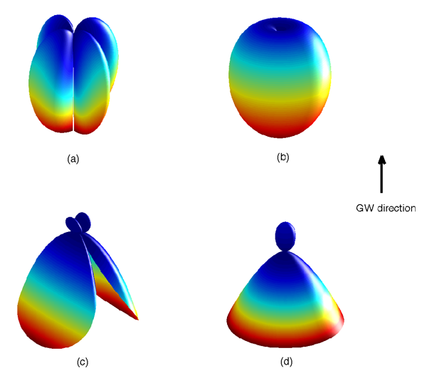
 -direction with the Earth at the origin, and the antenna pattern depends on the pulsar’s location.
The color indicates the strength of the response, red being the largest and blue the smallest.
-direction with the Earth at the origin, and the antenna pattern depends on the pulsar’s location.
The color indicates the strength of the response, red being the largest and blue the smallest.
 |
 |
 |
Living Rev. Relativity, 16 (2013), 9, doi:10.12942/lrr-2013-9, URL (accessed <date>): http://www.livingreviews.org/lrr-2013-9.
 This work is licensed under a Creative Commons License.
© The author(s), except where otherwise noted.
This work is licensed under a Creative Commons License.
© The author(s), except where otherwise noted.