Gamma distribution
From Wikipedia, the free encyclopedia
Probability density function |
|
Cumulative distribution function |
|
| Parameters |  shape (real) shape (real) scale (real) scale (real) |
| Support |  |
 |
|
| cdf |  |
| Mean |  |
| Median | |
| Mode |  for for  |
| Variance |  |
| Skewness |  |
| Kurtosis |  |
| Entropy |  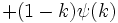 |
| mgf |  for t < 1 / θ for t < 1 / θ |
| Char. func. |  |
In probability theory and statistics, the gamma distribution is a continuous probability distribution. For integer values of the parameter k it is also known as the Erlang distribution.
Contents[hide] |
Probability density function
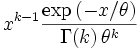
The probability density function of the gamma distribution can be expressed in terms of the gamma function:
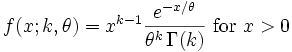
where k > 0 is the shape parameter and θ > 0 is the scale parameter of the gamma distribution. (NOTE: this parameterization is what is used in the infobox and the plots.)
Alternatively, the gamma distribution can be parameterized in terms of a shape parameter α = k and an inverse scale parameter β = 1 / θ, called a rate parameter:
Both parameterizations are common because they are convenient to use in certain situations and fields.
Properties
The cumulative distribution function can be expressed in terms of the incomplete gamma function,
The information entropy is given by:

where ψ(k) is the polygamma function.
If  for
for  and
and  then
then
![\left[ Y = \sum_{i=1}^N X_i \right] \sim \mathrm{Gamma} \left( \bar{\alpha}, \beta \right)](Gamma_distribution_files/ec639f8201ab44476a96b75cf9a810b9.png)
provided all Xi are independent. The gamma distribution exhibits infinite divisibility.
If  , then
 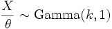 . Or, more generally, for any t > 0 it holds that
 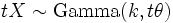 . That is the meaning of θ (or β) being the scale parameter.
Parameter estimation
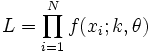
The likelihood function is
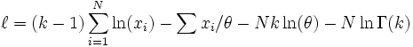
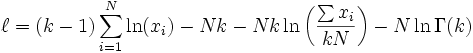
from which we calculate the log-likelihood function
Finding the maximum with respect to θ by taking the derivative and setting it equal to zero yields the maximum likelihood estimate of the θ parameter:
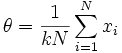
Substituting this into the log-likelihood function gives:
Finding the maximum with respect to k by taking the derivative and setting it equal to zero yields:
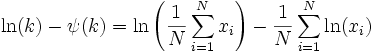
where 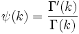 is the digamma function.
There is no closed-form solution for k. The function is numerically very well behaved, so if a numerical solution is desired, it can be found using Newton's method. An initial value of k can be found either using the method of moments, or using the approximation:
If we let  then k is approximately
which is within 1.5% of the correct value.
Generating Gamma random variables
Given the scaling property above, it is enough to generate Gamma variables with β = 1 as we can later convert to any value of β with simple division.
Using the fact that if  , then also
  , and the method of generating exponential variables, we conclude that if U is uniformly distributed on (0, 1], then
  . Now, using the "α-addition" property of Gamma distribution, we expand this result:
 ,
,
where Uk are all uniformly distributed on (0, 1 ] and independent.
All that is left now is to generate a variable distributed as  for 0 < δ < 1 and apply the "α-addition" property once more. This is the most difficult part, however.
We provide an algorithm without proof. It is an instance of the acceptance-rejection method:
- Let m be 1.
- Generate V2m − 1 and V2m — independent uniformly distributed on (0, 1] variables.
- If
 , where
  , then go to step 4, else go to step 5.
 - Let
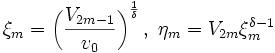 . Go to step 6.
 - Let
 .
. - If
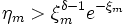 , then increment m and go to step 2.
 - Assume ξ = ξm to be the realization of .
Now, to summarize,
![\frac 1 \beta \left( \xi - \sum _{k=1} ^{[\alpha]} {\ln U_k} \right) \sim \operatorname{Gamma}(\alpha, \beta)](Gamma_distribution_files/8f8bfc0569478046512eccd87d5c7dc6.png) ,
,
where [α] is the integral part of α, ξ has been generating using the algorithm above with δ = {α} (the fractional part of α), Uk and Vl are distributed as explained above and are all independent.
Related distributions
 is an exponential distribution if
 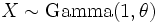 .
. if
if  for any c > 0 .
 is a gamma distribution if
 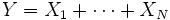 and if the
 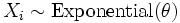 are all independent and share the same parameter θ.
 is a chi-square distribution if
  .
.- If k is an integer, the gamma distribution is an Erlang distribution (so named in honor of A. K. Erlang) and is the probability distribution of the waiting time until the k-th "arrival" in a one-dimensional Poisson process with intensity 1 / θ.
- then
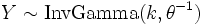 if Y = 1 / X, where InvGamma is the inverse-gamma distribution.
  is a beta distribution if
  < and
< and 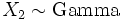 and are also independent.
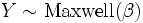 is a Maxwell-Boltzmann distribution if
  .
. is a normal distribution as
  where
where  .
.- The real vector
 follows a Dirichlet distribution if
 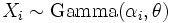 are independent, and
 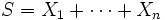 . This holds true for any θ.
References
- R. V. Hogg and A. T. Craig. Introduction to Mathematical Statistics, 4th edition. New York: Macmillan, 1978. (See Section 3.3.)

